

Physical Properties of Seawater 5.5 Temperature–Salinity Relationships 105
Part A | 5.5
is computed according to
pot D Â C 1000 ;
(5.7)
is based solely in terms of its surface temperature and
salinity.
One of the most important features of the ocean
is its vertical density gradient or stratification. In general, oceanic density increases with depth (i. e., z)
because there is the tendency for more dense parcels
to sink below less dense parcels. This density environment supports a restoring force (due to the density
difference and gravity) on a water parcel that has been
displaced from its equilibrium position, such that it
tends to its equilibrium position. The restoring force,
whose strength is related to the vertical potential density gradient, gives rise to a class of oscillations called
internal waves (discussed elsewhere). Oceanographers
express the strength of this restoring force in terms of
the buoyancy frequency, N or natural frequency of oscillation, given by
N.z/ D
s
g
@@ pot
@z
.in units of rad=s/ :
(5.8)
The vertical density gradient – corrected for the effects of compressibility – is the relevant quantity here.
If the more dense water is deeper, then the potential
density gradient is negative, the water column is stable, N is positive, and internal waves are possible. If
the water column density is uniform, then the potential density gradient and N are zero, the water column
is neutrally stable, and oscillations are not possible. If
more dense water sits atop less dense water, then the potential density gradient is positive, N is imaginary, the
water column is unstable, and short-term water column
overturning is inevitable.
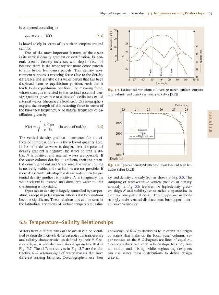
Open ocean density is largely controlled by temperature, except in polar regions where salinity variations
become significant. These relationships can be seen in
the latitudinal variations of surface temperature, salinTemperature (°C)
σ
t
Salinity (psu)
Tropic
Tropic
Equator
S 60°
40°
20°
20°
0°
40°
60°
80° N
Latitude
30
20
10
0
–5
28
26
24
22
36
35
34
33
32
Fig. 5.5 Latitudinal variations of average ocean surface temperature, salinity and density anomaly t (after [5.2])
Equator
Tropics
High latitude
23
24
25
26
27
28
Density σ t
Depth (m)
0
1000
2000
3000
4000
Fig. 5.6 Typical density/depth profiles at low and high latitudes (after [5.2])
ity, and density anomaly ( t ), as shown in Fig. 5.5. The
sampling of representative vertical profiles of density
anomaly in Fig. 5.6 features the high-density gradient (high N and stability) zone called a pycnocline in
the tropical/equatorial ocean. These upper ocean zones
strongly resist vertical displacement, but support internal wave variability.
5.5 Temperature–Salinity Relationships
Waters from different parts of the ocean can be identified by their distinctively different potential temperature
and salinity characteristics as defined by their  –S relationships, as revealed on a  –S diagram like that in
Fig. 5.7. The different curves in Fig. 5.7 are the distinctive  –S relationships of water masses that have
different mixing histories. Oceanographers use their
knowledge of  –S relationships to interpret the origin
of waters that make up the local water column. Superimposed on the  –S diagram are lines of equal t .
Oceanographers use such relationships to study water motion and mixing, while engineering designers
can use water mass distributions to define design
criteria.
Part A | 5.5
is computed according to
pot D Â C 1000 ;
(5.7)
is based solely in terms of its surface temperature and
salinity.
One of the most important features of the ocean
is its vertical density gradient or stratification. In general, oceanic density increases with depth (i. e., z)
because there is the tendency for more dense parcels
to sink below less dense parcels. This density environment supports a restoring force (due to the density
difference and gravity) on a water parcel that has been
displaced from its equilibrium position, such that it
tends to its equilibrium position. The restoring force,
whose strength is related to the vertical potential density gradient, gives rise to a class of oscillations called
internal waves (discussed elsewhere). Oceanographers
express the strength of this restoring force in terms of
the buoyancy frequency, N or natural frequency of oscillation, given by
N.z/ D
s
g
@@ pot
@z
.in units of rad=s/ :
(5.8)
The vertical density gradient – corrected for the effects of compressibility – is the relevant quantity here.
If the more dense water is deeper, then the potential
density gradient is negative, the water column is stable, N is positive, and internal waves are possible. If
the water column density is uniform, then the potential density gradient and N are zero, the water column
is neutrally stable, and oscillations are not possible. If
more dense water sits atop less dense water, then the potential density gradient is positive, N is imaginary, the
water column is unstable, and short-term water column
overturning is inevitable.
Open ocean density is largely controlled by temperature, except in polar regions where salinity variations
become significant. These relationships can be seen in
the latitudinal variations of surface temperature, salinTemperature (°C)
σ
t
Salinity (psu)
Tropic
Tropic
Equator
S 60°
40°
20°
20°
0°
40°
60°
80° N
Latitude
30
20
10
0
–5
28
26
24
22
36
35
34
33
32
Fig. 5.5 Latitudinal variations of average ocean surface temperature, salinity and density anomaly t (after [5.2])
Equator
Tropics
High latitude
23
24
25
26
27
28
Density σ t
Depth (m)
0
1000
2000
3000
4000
Fig. 5.6 Typical density/depth profiles at low and high latitudes (after [5.2])
ity, and density anomaly ( t ), as shown in Fig. 5.5. The
sampling of representative vertical profiles of density
anomaly in Fig. 5.6 features the high-density gradient (high N and stability) zone called a pycnocline in
the tropical/equatorial ocean. These upper ocean zones
strongly resist vertical displacement, but support internal wave variability.
5.5 Temperature–Salinity Relationships
Waters from different parts of the ocean can be identified by their distinctively different potential temperature
and salinity characteristics as defined by their  –S relationships, as revealed on a  –S diagram like that in
Fig. 5.7. The different curves in Fig. 5.7 are the distinctive  –S relationships of water masses that have
different mixing histories. Oceanographers use their
knowledge of  –S relationships to interpret the origin
of waters that make up the local water column. Superimposed on the  –S diagram are lines of equal t .
Oceanographers use such relationships to study water motion and mixing, while engineering designers
can use water mass distributions to define design
criteria.