

80
Multiscale Hydrologic Remote Sensing: Perspectives and Applications
flux estimation through the SEBAL and TSEB models, respectively, with different
input spatial resolutions. Results in Figure 4.10 show that SEBAL overestimates H if
compared with the one obtained using the higher pixel size resolutions. The overestimation causes an underestimation of instantaneous λET up to 100 W m –2 , reaching
1 mm day –1 in terms of ET d . The H overestimation is probably related to the choice
of boundary conditions that are not well defined at the lower resolution due to the
high spatial fragmentation of the landscape. This hypothesis is partially confirmed
by the increase in model errors with the reduction of spatial accuracy in the input
data (Cammalleri et al. 2009). Moreover, it is interesting to note that, contrary to that
modeled, the available energy is substantially insensitive to the input spatial resolution (not shown here). Results of the TSEB model do not show the same behavior.
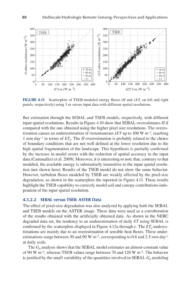
However, turbulent fluxes modeled by TSEB are weakly affected by the pixel-size
degradation, as shown in the scatterplots the reported in Figure 4.11. These results
highlight the TSEB capability to correctly model soil and canopy contributions independent of the input spatial resolution.
4.5.2.2 SEBAL versus TSEB: ASTER Data
The effect of pixel-size degradation was also analyzed by applying both the SEBAL
and TSEB models on the ASTER image. These data were used as a corroboration
of the results obtained with the artificially obtained data. As shown in the NERC
degraded data set, the tendency to an underestimation of daily ET using SEBAL is
confirmed by the scatterplots displayed in Figure 4.12a through c. The ET d underestimations are mainly due to an overestimation of sensible heat fluxes. These underestimations range between 50 and 90 W m –2 , corresponding to 0.8 and 2.5 mm day –1
at daily scale.
The G 0 analysis shows that the SEBAL model estimates an almost-constant value
of 90 W m –2 , whereas TSEB values range between 70 and 120 W m –2 . The behavior
is justified by the small variability of the quantities involved in SEBAL G 0 modeling
400
350
300
250
200
150
100
50
0 0
50 100 150 200 250 300 350 400
0
50 100 150 200 250 300 350 400
400
350
300
250
200
150
100
50
0
H other resolutions (W m –2
)
λET other resolutions (W m –2
)
H 3 m (W m –2 )
λET 3 m (W m –2 )
TSEB
TSEB
30 m
60 m
90 m
1:1
30 m
60 m
90 m
1:1
FIGURE 4.11 Scatterplots of TSEB-modeled energy fluxes (H and λET, on left and right
panels, respectively) using 3 m versus input data with different spatial resolutions.
Multiscale Hydrologic Remote Sensing: Perspectives and Applications
flux estimation through the SEBAL and TSEB models, respectively, with different
input spatial resolutions. Results in Figure 4.10 show that SEBAL overestimates H if
compared with the one obtained using the higher pixel size resolutions. The overestimation causes an underestimation of instantaneous λET up to 100 W m –2 , reaching
1 mm day –1 in terms of ET d . The H overestimation is probably related to the choice
of boundary conditions that are not well defined at the lower resolution due to the
high spatial fragmentation of the landscape. This hypothesis is partially confirmed
by the increase in model errors with the reduction of spatial accuracy in the input
data (Cammalleri et al. 2009). Moreover, it is interesting to note that, contrary to that
modeled, the available energy is substantially insensitive to the input spatial resolution (not shown here). Results of the TSEB model do not show the same behavior.
However, turbulent fluxes modeled by TSEB are weakly affected by the pixel-size
degradation, as shown in the scatterplots the reported in Figure 4.11. These results
highlight the TSEB capability to correctly model soil and canopy contributions independent of the input spatial resolution.
4.5.2.2 SEBAL versus TSEB: ASTER Data
The effect of pixel-size degradation was also analyzed by applying both the SEBAL
and TSEB models on the ASTER image. These data were used as a corroboration
of the results obtained with the artificially obtained data. As shown in the NERC
degraded data set, the tendency to an underestimation of daily ET using SEBAL is
confirmed by the scatterplots displayed in Figure 4.12a through c. The ET d underestimations are mainly due to an overestimation of sensible heat fluxes. These underestimations range between 50 and 90 W m –2 , corresponding to 0.8 and 2.5 mm day –1
at daily scale.
The G 0 analysis shows that the SEBAL model estimates an almost-constant value
of 90 W m –2 , whereas TSEB values range between 70 and 120 W m –2 . The behavior
is justified by the small variability of the quantities involved in SEBAL G 0 modeling
400
350
300
250
200
150
100
50
0 0
50 100 150 200 250 300 350 400
0
50 100 150 200 250 300 350 400
400
350
300
250
200
150
100
50
0
H other resolutions (W m –2
)
λET other resolutions (W m –2
)
H 3 m (W m –2 )
λET 3 m (W m –2 )
TSEB
TSEB
30 m
60 m
90 m
1:1
30 m
60 m
90 m
1:1
FIGURE 4.11 Scatterplots of TSEB-modeled energy fluxes (H and λET, on left and right
panels, respectively) using 3 m versus input data with different spatial resolutions.