

79
Comparative Analysis of Surface Energy Balance Models
20%. Finally, high MAD values were observable for the SEBAL model during the
first dates in fields C1 and C2; however, in this case, RE values are largely lower than
20% due to high flux magnitude.
The comparison on the whole scene highlights a good agreement among the results
of the three models, with MAD values almost always lower than the defined upper
limit. This result indicates that the high information content of the remotely sensed
images is sufficient to characterize the available energy partition, as quantified by
Λ, independently by the adopted approach, and that, in the analyzed case, both the
simplified and complex models accurately characterize the average water stress at the
scene scale. Yet, higher discrepancies are evident over fields characterized by low vegetation coverage and high atmospheric water demand. In correspondence of the last
two acquisitions, carried out after two rainfall events, the water availability increase
made negligible the discrepancies among models in terms of both MAD and RE.
4.5.2 analySiS of the Pixel-Size effect
On the basis of the results previously shown, the successive analyses were focused
only on the residual energy balance approaches SEBAL and TSEB. For this reason,
the two models were applied based on two sets of data acquired by airborne and satellite platforms as previously reported. Models’ outputs were analyzed and compared
in terms of pixel-by-pixel scatterplots. The pixel-size effect was analyzed by applying
the models to the NERC airborne images aggregated to different resolutions up to
the ASTER satellite ones (90 m × 90 m). Finally, results obtained with the artificially
degraded data were compared with the one retrieved with actual ASTER data.
4.5.2.1 SEBAL versus TSEB: NERC Data
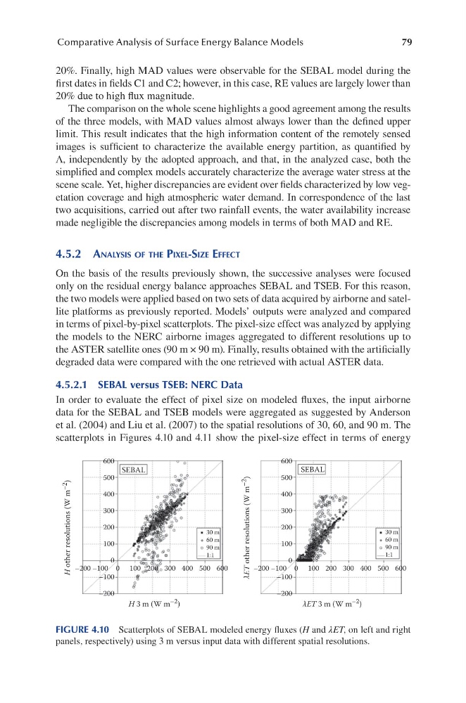
In order to evaluate the effect of pixel size on modeled fluxes, the input airborne
data for the SEBAL and TSEB models were aggregated as suggested by Anderson
et al. (2004) and Liu et al. (2007) to the spatial resolutions of 30, 60, and 90 m. The
scatterplots in Figures 4.10 and 4.11 show the pixel-size effect in terms of energy
600
500
400
300
200
100
–100
–200
–200 –100
100
H 3 m (W m –2 )
H other resolutions (W m –2
)
λET other resolutions (W m –2
)
λET 3 m (W m –2 )
200 300 400 500 600
0
–200 –100
100 200 300 400 500 600
0
0
600
500
400
300
200
100
–100
–200
0
SEBAL
SEBAL
30 m
60 m
90 m
1:1
30 m
60 m
90 m
1:1
FIGURE 4.10 Scatterplots of SEBAL modeled energy fluxes (H and λET, on left and right
panels, respectively) using 3 m versus input data with different spatial resolutions.
Comparative Analysis of Surface Energy Balance Models
20%. Finally, high MAD values were observable for the SEBAL model during the
first dates in fields C1 and C2; however, in this case, RE values are largely lower than
20% due to high flux magnitude.
The comparison on the whole scene highlights a good agreement among the results
of the three models, with MAD values almost always lower than the defined upper
limit. This result indicates that the high information content of the remotely sensed
images is sufficient to characterize the available energy partition, as quantified by
Λ, independently by the adopted approach, and that, in the analyzed case, both the
simplified and complex models accurately characterize the average water stress at the
scene scale. Yet, higher discrepancies are evident over fields characterized by low vegetation coverage and high atmospheric water demand. In correspondence of the last
two acquisitions, carried out after two rainfall events, the water availability increase
made negligible the discrepancies among models in terms of both MAD and RE.
4.5.2 analySiS of the Pixel-Size effect
On the basis of the results previously shown, the successive analyses were focused
only on the residual energy balance approaches SEBAL and TSEB. For this reason,
the two models were applied based on two sets of data acquired by airborne and satellite platforms as previously reported. Models’ outputs were analyzed and compared
in terms of pixel-by-pixel scatterplots. The pixel-size effect was analyzed by applying
the models to the NERC airborne images aggregated to different resolutions up to
the ASTER satellite ones (90 m × 90 m). Finally, results obtained with the artificially
degraded data were compared with the one retrieved with actual ASTER data.
4.5.2.1 SEBAL versus TSEB: NERC Data
In order to evaluate the effect of pixel size on modeled fluxes, the input airborne
data for the SEBAL and TSEB models were aggregated as suggested by Anderson
et al. (2004) and Liu et al. (2007) to the spatial resolutions of 30, 60, and 90 m. The
scatterplots in Figures 4.10 and 4.11 show the pixel-size effect in terms of energy
600
500
400
300
200
100
–100
–200
–200 –100
100
H 3 m (W m –2 )
H other resolutions (W m –2
)
λET other resolutions (W m –2
)
λET 3 m (W m –2 )
200 300 400 500 600
0
–200 –100
100 200 300 400 500 600
0
0
600
500
400
300
200
100
–100
–200
0
SEBAL
SEBAL
30 m
60 m
90 m
1:1
30 m
60 m
90 m
1:1
FIGURE 4.10 Scatterplots of SEBAL modeled energy fluxes (H and λET, on left and right
panels, respectively) using 3 m versus input data with different spatial resolutions.