

76
Multiscale Hydrologic Remote Sensing: Perspectives and Applications
plots in Figures 4.8 and 4.9 report both MAD and RE values obtained for the five
analyzed fields and the whole scene during the entire period. In particular, Figure
4.8 shows the MAD values of SEBAL and S-SEBI (assuming TSEB outputs as ref.8 shows the MAD values of SEBAL and S-SEBI (assuming TSEB outputs as reference). The analysis of the bar plots in Figure 4.8 highlights some discrepancies
occurring in the vineyard (in particular, within the field V1) associated with the first
10.0
ET
d (mm day –1
)
8.0
6.0
4.0
2.0
0.0
–2.0
10.0
ET
d (mm day –1
)
8.0
6.0
4.0
2.0
0.0
–2.0
10.0
ET
d (mm day –1
)
8.0
6.0
4.0
2.0
0.0
–2.0
10.0
ET
d (mm day –1
)
8.0
6.0
4.0
2.0
0.0
–2.0
C1
C2
O
V1
V2
ALL
C1
C2
O
V1
V2
ALL
C1
C2
O
V1
V2
ALL
C1
C2
O
V1
V2
ALL
C1
C2
O
V1
V2
ALL
C1
C2
O
V1
V2
ALL
C1
C2
O
V1
V2
ALL
C1
C2
O
V1
V2
ALL
Field
Field
DOY 163
DOY 185
DOY 204
DOY 235
DOY 247
SEBAL
TSEB
S-SEBI
DOY 284
DOY 295
Mean
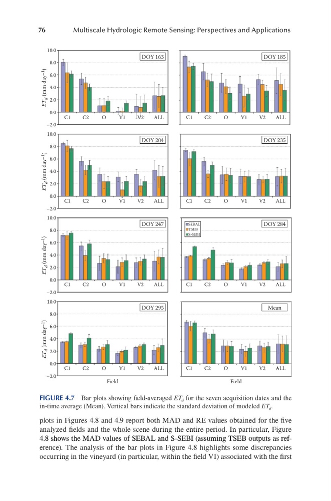
FIGURE 4.7 Bar plots showing field-averaged ET d for the seven acquisition dates and the
in-time average (Mean). Vertical bars indicate the standard deviation of modeled ET d .
Multiscale Hydrologic Remote Sensing: Perspectives and Applications
plots in Figures 4.8 and 4.9 report both MAD and RE values obtained for the five
analyzed fields and the whole scene during the entire period. In particular, Figure
4.8 shows the MAD values of SEBAL and S-SEBI (assuming TSEB outputs as ref.8 shows the MAD values of SEBAL and S-SEBI (assuming TSEB outputs as reference). The analysis of the bar plots in Figure 4.8 highlights some discrepancies
occurring in the vineyard (in particular, within the field V1) associated with the first
10.0
ET
d (mm day –1
)
8.0
6.0
4.0
2.0
0.0
–2.0
10.0
ET
d (mm day –1
)
8.0
6.0
4.0
2.0
0.0
–2.0
10.0
ET
d (mm day –1
)
8.0
6.0
4.0
2.0
0.0
–2.0
10.0
ET
d (mm day –1
)
8.0
6.0
4.0
2.0
0.0
–2.0
C1
C2
O
V1
V2
ALL
C1
C2
O
V1
V2
ALL
C1
C2
O
V1
V2
ALL
C1
C2
O
V1
V2
ALL
C1
C2
O
V1
V2
ALL
C1
C2
O
V1
V2
ALL
C1
C2
O
V1
V2
ALL
C1
C2
O
V1
V2
ALL
Field
Field
DOY 163
DOY 185
DOY 204
DOY 235
DOY 247
SEBAL
TSEB
S-SEBI
DOY 284
DOY 295
Mean
FIGURE 4.7 Bar plots showing field-averaged ET d for the seven acquisition dates and the
in-time average (Mean). Vertical bars indicate the standard deviation of modeled ET d .