

75
Comparative Analysis of Surface Energy Balance Models
outputs in terms of spatial distribution. The analysis highlights a substantial agreement
among the three ET d maps, with only slight differences over bare soil in the upper part
of the study area in the case of S-SEBI.
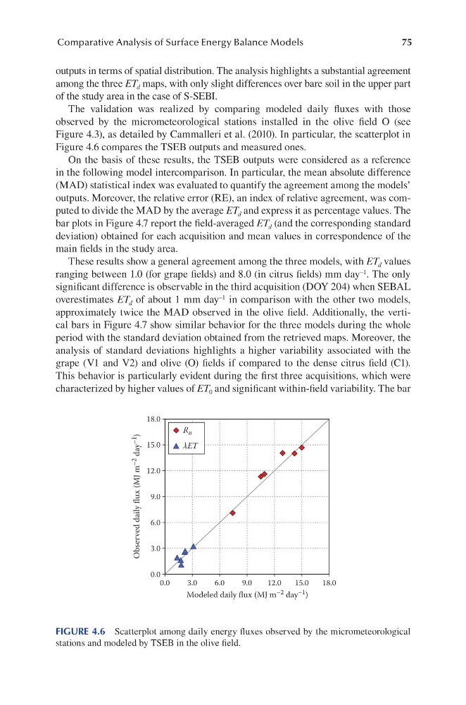
The validation was realized by comparing modeled daily fluxes with those
observed by the micrometeorological stations installed in the olive field O (see
Figure 4.3), as detailed by Cammalleri et al. (2010). In particular, the scatterplot in
Figure 4.6 compares the TSEB outputs and measured ones.
On the basis of these results, the TSEB outputs were considered as a reference
in the following model intercomparison. In particular, the mean absolute difference
(MAD) statistical index was evaluated to quantify the agreement among the models’
outputs. Moreover, the relative error (RE), an index of relative agreement, was computed to divide the MAD by the average ET d and express it as percentage values. The
bar plots in Figure 4.7 report the field-averaged ET d (and the corresponding standard
deviation) obtained for each acquisition and mean values in correspondence of the
main fields in the study area.
These results show a general agreement among the three models, with ET d values
ranging between 1.0 (for grape fields) and 8.0 (in citrus fields) mm day –1 . The only
significant difference is observable in the third acquisition (DOY 204) when SEBAL
overestimates ET d of about 1 mm day –1 in comparison with the other two models,
approximately twice the MAD observed in the olive field. Additionally, the vertical bars in Figure 4.7 show similar behavior for the three models during the whole
period with the standard deviation obtained from the retrieved maps. Moreover, the
analysis of standard deviations highlights a higher variability associated with the
grape (V1 and V2) and olive (O) fields if compared to the dense citrus field (C1).
This behavior is particularly evident during the first three acquisitions, which were
characterized by higher values of ET 0 and significant within-field variability. The bar
18.0
15.0
12.0
9.0
6.0
3.0
0.0
0.0
3.0
6.0
9.0
12.0
15.0
18.0
Modeled daily flux (MJ m –2 day –1 )
Observed daily flux (MJ m –2
day –1
)
R n
λET
FIGURE 4.6 Scatterplot among daily energy fluxes observed by the micrometeorological
stations and modeled by TSEB in the olive field.
Comparative Analysis of Surface Energy Balance Models
outputs in terms of spatial distribution. The analysis highlights a substantial agreement
among the three ET d maps, with only slight differences over bare soil in the upper part
of the study area in the case of S-SEBI.
The validation was realized by comparing modeled daily fluxes with those
observed by the micrometeorological stations installed in the olive field O (see
Figure 4.3), as detailed by Cammalleri et al. (2010). In particular, the scatterplot in
Figure 4.6 compares the TSEB outputs and measured ones.
On the basis of these results, the TSEB outputs were considered as a reference
in the following model intercomparison. In particular, the mean absolute difference
(MAD) statistical index was evaluated to quantify the agreement among the models’
outputs. Moreover, the relative error (RE), an index of relative agreement, was computed to divide the MAD by the average ET d and express it as percentage values. The
bar plots in Figure 4.7 report the field-averaged ET d (and the corresponding standard
deviation) obtained for each acquisition and mean values in correspondence of the
main fields in the study area.
These results show a general agreement among the three models, with ET d values
ranging between 1.0 (for grape fields) and 8.0 (in citrus fields) mm day –1 . The only
significant difference is observable in the third acquisition (DOY 204) when SEBAL
overestimates ET d of about 1 mm day –1 in comparison with the other two models,
approximately twice the MAD observed in the olive field. Additionally, the vertical bars in Figure 4.7 show similar behavior for the three models during the whole
period with the standard deviation obtained from the retrieved maps. Moreover, the
analysis of standard deviations highlights a higher variability associated with the
grape (V1 and V2) and olive (O) fields if compared to the dense citrus field (C1).
This behavior is particularly evident during the first three acquisitions, which were
characterized by higher values of ET 0 and significant within-field variability. The bar
18.0
15.0
12.0
9.0
6.0
3.0
0.0
0.0
3.0
6.0
9.0
12.0
15.0
18.0
Modeled daily flux (MJ m –2 day –1 )
Observed daily flux (MJ m –2
day –1
)
R n
λET
FIGURE 4.6 Scatterplot among daily energy fluxes observed by the micrometeorological
stations and modeled by TSEB in the olive field.