

49
Storm Impact on the Coastal Geomorphology and Current Field
The water level record proves the impact of both wind stress and air pressure on
the water level, as seen in Figure 3.7 (lower panel). During the westerly strong winds
(February 22–23), the air pressure is constant, but the water level measurement is 1.5
and 2 m above the mean sea water level despite the neap tide. The difference of the high
water with the astronomical prediction varies between 1 and 1.5 m. During the last part
of the storm (February 26–27), the synergy of the trespassing of the extreme low front
with the westerly wind prevented the ebb phase of the tide. Because of this, the flooding
phase lasted 18 h. The correlation of the water level with air pressure proved that the
decrease in air pressure caused the continuous flooding. After stabilization of the air
pressure, the normal behavior of the tidal cycle was reestablished. In general, the impact
of air pressure variation on the water level has been broadly discussed during the last
two centuries, for example, by Ross (1854) and Doodson (1924), who introduced the
terminology “inverted barometer response” (Proudman 1929; Munk and MacDonald
1960; Wunsch 1972; Dickman 1988; Ponte 1994; and many others; a review could be
retrieved from the work of Wunsch and Stammer 1997), and still, there is ongoing
research. All of these publications are based on water-level measurements or modeling,
but herein, the subject is the response of the current field at the mouth of the tidal inlet.
3.5.2 StoRM iMPact on the BathyMetRy
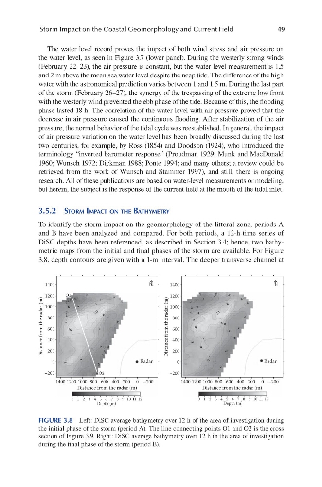
To identify the storm impact on the geomorphology of the littoral zone, periods A
and B have been analyzed and compared. For both periods, a 12-h time series of
DiSC depths have been referenced, as described in Section 3.4; hence, two bathymetric maps from the initial and final phases of the storm are available. For Figure
3.8, depth contours are given with a 1-m interval. The deeper transverse channel at
1400
1200
1000
800
600
400
200
0
–200
1400 1200 1000 800
0 1 2 3 4 5 6 7
Depth (m)
8 9 10 11 12
0 1 2 3 4 5 6 7
Depth (m)
8 9 10 11 12
600
Distance from the radar (m)
Radar
Radar
Distance from the radar (m)
Distance from the radar (m)
Distance from the radar (m)
400 200 0 –200
1400
1200
1000
800
600
400
200
0
–200
1400 1200 1000 800 600 400 200 0 –200
O1
O2
7
8
8
7
7
7
6
9
8
1 0
1 0
9
9
6
6
7
8
9
9
8
5
5
5
5
6
6
5
5
4
4
4
7
7
7
7
7
7
6
6
6
6
6
5 5
5
8
8
8
8
8
8
10
1 0
8
9
9
9
9
8
8
5 9
6
FIGURE 3.8 Left: DiSC average bathymetry over 12 h of the area of investigation during
the initial phase of the storm (period A). The line connecting points O1 and O2 is the cross
section of Figure 3.9. Right: DiSC average bathymetry over 12 h in the area of investigation
during the final phase of the storm (period B).
Storm Impact on the Coastal Geomorphology and Current Field
The water level record proves the impact of both wind stress and air pressure on
the water level, as seen in Figure 3.7 (lower panel). During the westerly strong winds
(February 22–23), the air pressure is constant, but the water level measurement is 1.5
and 2 m above the mean sea water level despite the neap tide. The difference of the high
water with the astronomical prediction varies between 1 and 1.5 m. During the last part
of the storm (February 26–27), the synergy of the trespassing of the extreme low front
with the westerly wind prevented the ebb phase of the tide. Because of this, the flooding
phase lasted 18 h. The correlation of the water level with air pressure proved that the
decrease in air pressure caused the continuous flooding. After stabilization of the air
pressure, the normal behavior of the tidal cycle was reestablished. In general, the impact
of air pressure variation on the water level has been broadly discussed during the last
two centuries, for example, by Ross (1854) and Doodson (1924), who introduced the
terminology “inverted barometer response” (Proudman 1929; Munk and MacDonald
1960; Wunsch 1972; Dickman 1988; Ponte 1994; and many others; a review could be
retrieved from the work of Wunsch and Stammer 1997), and still, there is ongoing
research. All of these publications are based on water-level measurements or modeling,
but herein, the subject is the response of the current field at the mouth of the tidal inlet.
3.5.2 StoRM iMPact on the BathyMetRy
To identify the storm impact on the geomorphology of the littoral zone, periods A
and B have been analyzed and compared. For both periods, a 12-h time series of
DiSC depths have been referenced, as described in Section 3.4; hence, two bathymetric maps from the initial and final phases of the storm are available. For Figure
3.8, depth contours are given with a 1-m interval. The deeper transverse channel at
1400
1200
1000
800
600
400
200
0
–200
1400 1200 1000 800
0 1 2 3 4 5 6 7
Depth (m)
8 9 10 11 12
0 1 2 3 4 5 6 7
Depth (m)
8 9 10 11 12
600
Distance from the radar (m)
Radar
Radar
Distance from the radar (m)
Distance from the radar (m)
Distance from the radar (m)
400 200 0 –200
1400
1200
1000
800
600
400
200
0
–200
1400 1200 1000 800 600 400 200 0 –200
O1
O2
7
8
8
7
7
7
6
9
8
1 0
1 0
9
9
6
6
7
8
9
9
8
5
5
5
5
6
6
5
5
4
4
4
7
7
7
7
7
7
6
6
6
6
6
5 5
5
8
8
8
8
8
8
10
1 0
8
9
9
9
9
8
8
5 9
6
FIGURE 3.8 Left: DiSC average bathymetry over 12 h of the area of investigation during
the initial phase of the storm (period A). The line connecting points O1 and O2 is the cross
section of Figure 3.9. Right: DiSC average bathymetry over 12 h in the area of investigation
during the final phase of the storm (period B).