

281
Precipitation Estimate Using NEXRAD Ground-Based Radar Images
where ˆ
β β GLS is the GLS estimate of (β 0 ,β 1 ), and C ε (x i ,x j ) is the covariance of residuals
of point pairs (x i ,x j ). The GLS method was suggested to estimate the trend through
an iterative means. The ordinary least squares (OLS) estimates are obtained, and a
variogram is fitted to the residuals. This variogram is then used in the GLS regression method to reestimate the trend. These procedures are repeated until the estimates stabilize. The convergence of this iterative GLS process may require much
time and computational resources. Practically, a single iteration can be used as a
satisfactory solution (Kitanidis 1994). In this study, three iterations were adopted to
estimate the GLS residuals.
12.3.2.5 Kriging with External Drift
In RK, the trend of the random variable is constant. While in real-world problems,
some spatial processes include varying trend or “drift” (Webster and Oliver 2007),
in KED, the trend m(x) of the random variable is not stationary, which can take into
account both the spatial dependence of the variable and its linear relation to one or
more additional variables (Ahmed and De Marsily 1987). The form of m(x) in KED
is the same as that in RK; however, the coefficients β k are unknown coefficients to
be determined. The expression for the KED estimate of Z(u) is the same as that of
OK, but the equation system used to obtain the optimal weights of KED is different.
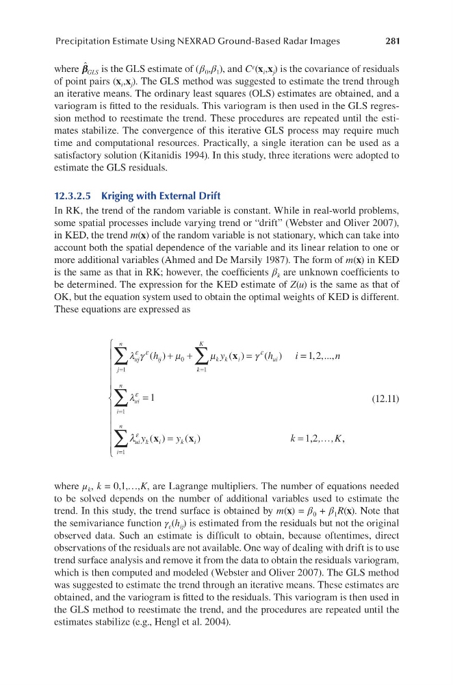
These equations are expressed as
λ γ
µ
µ
γ
ε ε
ε
uj
j
n
ij
k k
i
k
K
ui
h
y
h
i
=
=
∑
∑
+ +
=
1
0
1
( )
( )
( )
x
= =
=
=
=
=
∑
∑
1 2
1
1
, ,...,
( )
( )
n
y
y
ui
i
n
ui k
i
k
i
i
n
λ
ε
ε
λ
1
x
x
1,2
,
k
, ,K
=
…
(12.11)
where μ k , k = 0,1,…,K, are Lagrange multipliers. The number of equations needed
to be solved depends on the number of additional variables used to estimate the
trend. In this study, the trend surface is obtained by m(x) = β 0 + β 1 R(x). Note that
the semivariance function γ ε (h ij ) is estimated from the residuals but not the original
observed data. Such an estimate is difficult to obtain, because oftentimes, direct
observations of the residuals are not available. One way of dealing with drift is to use
trend surface analysis and remove it from the data to obtain the residuals variogram,
which is then computed and modeled (Webster and Oliver 2007). The GLS method
was suggested to estimate the trend through an iterative means. These estimates are
obtained, and the variogram is fitted to the residuals. This variogram is then used in
the GLS method to reestimate the trend, and the procedures are repeated until the
estimates stabilize (e.g., Hengl et al. 2004).
Precipitation Estimate Using NEXRAD Ground-Based Radar Images
where ˆ
β β GLS is the GLS estimate of (β 0 ,β 1 ), and C ε (x i ,x j ) is the covariance of residuals
of point pairs (x i ,x j ). The GLS method was suggested to estimate the trend through
an iterative means. The ordinary least squares (OLS) estimates are obtained, and a
variogram is fitted to the residuals. This variogram is then used in the GLS regression method to reestimate the trend. These procedures are repeated until the estimates stabilize. The convergence of this iterative GLS process may require much
time and computational resources. Practically, a single iteration can be used as a
satisfactory solution (Kitanidis 1994). In this study, three iterations were adopted to
estimate the GLS residuals.
12.3.2.5 Kriging with External Drift
In RK, the trend of the random variable is constant. While in real-world problems,
some spatial processes include varying trend or “drift” (Webster and Oliver 2007),
in KED, the trend m(x) of the random variable is not stationary, which can take into
account both the spatial dependence of the variable and its linear relation to one or
more additional variables (Ahmed and De Marsily 1987). The form of m(x) in KED
is the same as that in RK; however, the coefficients β k are unknown coefficients to
be determined. The expression for the KED estimate of Z(u) is the same as that of
OK, but the equation system used to obtain the optimal weights of KED is different.
These equations are expressed as
λ γ
µ
µ
γ
ε ε
ε
uj
j
n
ij
k k
i
k
K
ui
h
y
h
i
=
=
∑
∑
+ +
=
1
0
1
( )
( )
( )
x
= =
=
=
=
=
∑
∑
1 2
1
1
, ,...,
( )
( )
n
y
y
ui
i
n
ui k
i
k
i
i
n
λ
ε
ε
λ
1
x
x
1,2
,
k
, ,K
=
…
(12.11)
where μ k , k = 0,1,…,K, are Lagrange multipliers. The number of equations needed
to be solved depends on the number of additional variables used to estimate the
trend. In this study, the trend surface is obtained by m(x) = β 0 + β 1 R(x). Note that
the semivariance function γ ε (h ij ) is estimated from the residuals but not the original
observed data. Such an estimate is difficult to obtain, because oftentimes, direct
observations of the residuals are not available. One way of dealing with drift is to use
trend surface analysis and remove it from the data to obtain the residuals variogram,
which is then computed and modeled (Webster and Oliver 2007). The GLS method
was suggested to estimate the trend through an iterative means. These estimates are
obtained, and the variogram is fitted to the residuals. This variogram is then used in
the GLS method to reestimate the trend, and the procedures are repeated until the
estimates stabilize (e.g., Hengl et al. 2004).