

280
Multiscale Hydrologic Remote Sensing: Perspectives and Applications
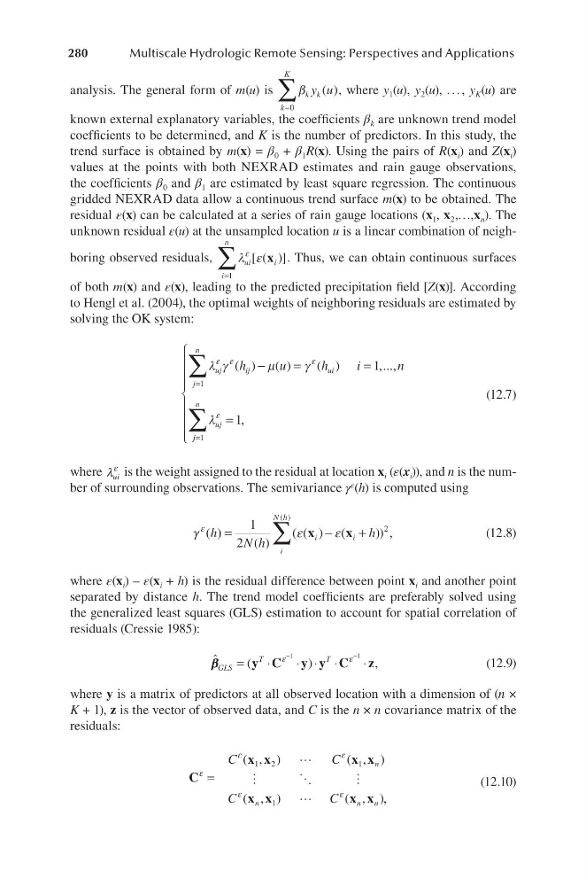
analysis. The general form of m(u) is
β k k
k
K
y u
( )
=
∑
0
, where y 1 (u), y 2 (u), . . . , y K (u) are
known external explanatory variables, the coefficients β k are unknown trend model
coefficients to be determined, and K is the number of predictors. In this study, the
trend surface is obtained by m(x) = β 0 + β 1 R(x). Using the pairs of R(x i ) and Z(x i )
values at the points with both NEXRAD estimates and rain gauge observations,
the coefficients β 0 and β 1 are estimated by least square regression. The continuous
gridded NEXRAD data allow a continuous trend surface m(x) to be obtained. The
residual ε(x) can be calculated at a series of rain gauge locations (x 1 , x 2 ,…,x n ). The
unknown residual ε(u) at the unsampled location u is a linear combination of neighboring observed residuals,
λ ε
ε
ui
i
n
i
=
∑
1
[ ( )]
x . Thus, we can obtain continuous surfaces
of both m(x) and ε(x), leading to the predicted precipitation field [Z(x)]. According
to Hengl et al. (2004), the optimal weights of neighboring residuals are estimated by
solving the OK system:
λ γ
µ
γ
λ
ε ε
ε
ε
uj
j
n
ij
ui
uj
h
u
h
i
n
=
∑
−
=
=
1
1
( ) ( )
( )
,...,
j j
n
=
∑ =
1
1,
(12.7)
where λ
ε
ui is the weight assigned to the residual at location x i (ε(x i )), and n is the number of surrounding observations. The semivariance γ ε (h) is computed using
γ
ε
ε
ε ( )
( )
( ( ) (
)) ,
( )
h
N h
h
i
i
i
N h
=
−
+
∑
1
2
2
x
x
(12.8)
where ε(x i ) – ε(x i + h) is the residual difference between point x i and another point
separated by distance h. The trend model coefficients are preferably solved using
the generalized least squares (GLS) estimation to account for spatial correlation of
residuals (Cressie 1985):
ˆ
(
)
β β GLS
T
T
=
⋅
⋅ ⋅ ⋅
⋅
−
−
y C y y C z
ε
ε
1
1
,
(12.9)
where y is a matrix of predictors at all observed location with a dimension of (n ×
K + 1), z is the vector of observed data, and C is the n × n covariance matrix of the
residuals:
C
x x
x x
x x
x x
ε
ε
ε
ε
ε
=
C
C
C
C
n
n
n
n
( , )
( , )
( , )
( , ),
1
2
1
1
(12.10)
Multiscale Hydrologic Remote Sensing: Perspectives and Applications
analysis. The general form of m(u) is
β k k
k
K
y u
( )
=
∑
0
, where y 1 (u), y 2 (u), . . . , y K (u) are
known external explanatory variables, the coefficients β k are unknown trend model
coefficients to be determined, and K is the number of predictors. In this study, the
trend surface is obtained by m(x) = β 0 + β 1 R(x). Using the pairs of R(x i ) and Z(x i )
values at the points with both NEXRAD estimates and rain gauge observations,
the coefficients β 0 and β 1 are estimated by least square regression. The continuous
gridded NEXRAD data allow a continuous trend surface m(x) to be obtained. The
residual ε(x) can be calculated at a series of rain gauge locations (x 1 , x 2 ,…,x n ). The
unknown residual ε(u) at the unsampled location u is a linear combination of neighboring observed residuals,
λ ε
ε
ui
i
n
i
=
∑
1
[ ( )]
x . Thus, we can obtain continuous surfaces
of both m(x) and ε(x), leading to the predicted precipitation field [Z(x)]. According
to Hengl et al. (2004), the optimal weights of neighboring residuals are estimated by
solving the OK system:
λ γ
µ
γ
λ
ε ε
ε
ε
uj
j
n
ij
ui
uj
h
u
h
i
n
=
∑
−
=
=
1
1
( ) ( )
( )
,...,
j j
n
=
∑ =
1
1,
(12.7)
where λ
ε
ui is the weight assigned to the residual at location x i (ε(x i )), and n is the number of surrounding observations. The semivariance γ ε (h) is computed using
γ
ε
ε
ε ( )
( )
( ( ) (
)) ,
( )
h
N h
h
i
i
i
N h
=
−
+
∑
1
2
2
x
x
(12.8)
where ε(x i ) – ε(x i + h) is the residual difference between point x i and another point
separated by distance h. The trend model coefficients are preferably solved using
the generalized least squares (GLS) estimation to account for spatial correlation of
residuals (Cressie 1985):
ˆ
(
)
β β GLS
T
T
=
⋅
⋅ ⋅ ⋅
⋅
−
−
y C y y C z
ε
ε
1
1
,
(12.9)
where y is a matrix of predictors at all observed location with a dimension of (n ×
K + 1), z is the vector of observed data, and C is the n × n covariance matrix of the
residuals:
C
x x
x x
x x
x x
ε
ε
ε
ε
ε
=
C
C
C
C
n
n
n
n
( , )
( , )
( , )
( , ),
1
2
1
1
(12.10)