

279
Precipitation Estimate Using NEXRAD Ground-Based Radar Images
2008) showed that the performance of kriging methods can be improved by using
external information to estimate m(x).
In OK, a common type of kriging practice, the trend is considered unknown and
constant. OK estimates the unknown precipitation depth at the unsampled location
u as a linear combination of neighboring observations: Z u
Z
ui
i
n
i
( )
[ ( )]
=
=
∑ λ
1
x . The
optimal weights are obtained through solving a series of linear functions known as
the OK system (Goovaerts 2000):
λ γ
µ
γ
λ
uj
j
n
ij
ui
uj
j
n
h
u
h
i
n
=
=
∑
−
=
=
1
1
1
( ) ( )
( )
,...,
∑ ∑ =
1,
(12.4)
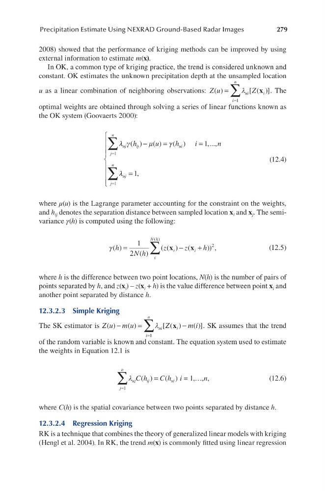
where μ(u) is the Lagrange parameter accounting for the constraint on the weights,
and h ij denotes the separation distance between sampled location x i and x j . The semivariance γ(h) is computed using the following:
γ ( )
( )
( ( ) (
)) ,
( )
h
N h
z
z
h
i
i
i
N h
=
−
+
∑
1
2
2
x
x
(12.5)
where h is the difference between two point locations, N(h) is the number of pairs of
points separated by h, and z(x i ) – z(x i + h) is the value difference between point x i and
another point separated by distance h.
12.3.2.3 Simple Kriging
The SK estimator is Z u m u
Z
m i
ui
i
n
i
( )
( )
[ ( )
( )]
−
=
−
=
∑ λ
1
x
. SK assumes that the trend
of the random variable is known and constant. The equation system used to estimate
the weights in Equation 12.1 is
λ uj
j
n
ij
ui
C h
C h
=
∑
=
1
( )
( ) i = 1,…,n,
(12.6)
where C(h) is the spatial covariance between two points separated by distance h.
12.3.2.4 Regression Kriging
RK is a technique that combines the theory of generalized linear models with kriging
(Hengl et al. 2004). In RK, the trend m(x) is commonly fitted using linear regression
Precipitation Estimate Using NEXRAD Ground-Based Radar Images
2008) showed that the performance of kriging methods can be improved by using
external information to estimate m(x).
In OK, a common type of kriging practice, the trend is considered unknown and
constant. OK estimates the unknown precipitation depth at the unsampled location
u as a linear combination of neighboring observations: Z u
Z
ui
i
n
i
( )
[ ( )]
=
=
∑ λ
1
x . The
optimal weights are obtained through solving a series of linear functions known as
the OK system (Goovaerts 2000):
λ γ
µ
γ
λ
uj
j
n
ij
ui
uj
j
n
h
u
h
i
n
=
=
∑
−
=
=
1
1
1
( ) ( )
( )
,...,
∑ ∑ =
1,
(12.4)
where μ(u) is the Lagrange parameter accounting for the constraint on the weights,
and h ij denotes the separation distance between sampled location x i and x j . The semivariance γ(h) is computed using the following:
γ ( )
( )
( ( ) (
)) ,
( )
h
N h
z
z
h
i
i
i
N h
=
−
+
∑
1
2
2
x
x
(12.5)
where h is the difference between two point locations, N(h) is the number of pairs of
points separated by h, and z(x i ) – z(x i + h) is the value difference between point x i and
another point separated by distance h.
12.3.2.3 Simple Kriging
The SK estimator is Z u m u
Z
m i
ui
i
n
i
( )
( )
[ ( )
( )]
−
=
−
=
∑ λ
1
x
. SK assumes that the trend
of the random variable is known and constant. The equation system used to estimate
the weights in Equation 12.1 is
λ uj
j
n
ij
ui
C h
C h
=
∑
=
1
( )
( ) i = 1,…,n,
(12.6)
where C(h) is the spatial covariance between two points separated by distance h.
12.3.2.4 Regression Kriging
RK is a technique that combines the theory of generalized linear models with kriging
(Hengl et al. 2004). In RK, the trend m(x) is commonly fitted using linear regression