

175
Modeling Stream Flow Changes
of the connections (weights) between elements until the network output matches the
target. In this study, we use a feedforward network with the default tan-sigmoid
transfer function in the hidden layer:
f(x) = [1 + exp(–x)] –1 .
(8.2)
In practice, many neural network modeling tools are available. In this study, the
MATLAB ® neural network fitting tool was applied, which solves the input–output
fitting problem with a two-layer neural network model. In this analysis, the input
variables include the time series data of temperature and precipitation collected at
six points. In the training period, three hidden layers were chosen, and the train. In the training period, three hidden layers were chosen, and the trainIn the training period, three hidden layers were chosen, and the training performance was evaluated using mean square error and regression analysis.
Overfitting has to be avoided when splitting the data sets for training and verification.
8.4 RESULTS
8.4.1 outPut of the eof analySiS
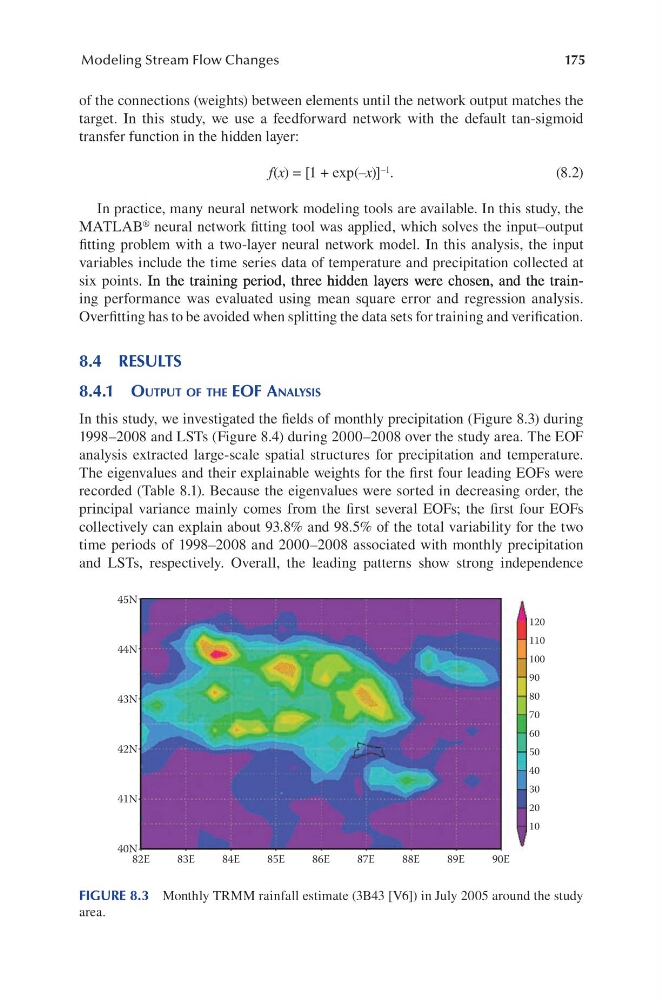
In this study, we investigated the fields of monthly precipitation (Figure 8.3) during
1998–2008 and LSTs (Figure 8.4) during 2000–2008 over the study area. The EOF
analysis extracted large-scale spatial structures for precipitation and temperature.
The eigenvalues and their explainable weights for the first four leading EOFs were
recorded (Table 8.1). Because the eigenvalues were sorted in decreasing order, the
principal variance mainly comes from the first several EOFs; the first four EOFs
collectively can explain about 93.8% and 98.5% of the total variability for the two
time periods of 1998–2008 and 2000–2008 associated with monthly precipitation
and LSTs, respectively. Overall, the leading patterns show strong independence
45N
44N
43N
42N
41N
40N
82E
83E
84E
85E
86E
87E
88E
89E
90E
120
110
100
90
80
70
60
50
40
30
20
10
FIGURE 8.3 Monthly TRMM rainfall estimate (3B43 [V6]) in July 2005 around the study
area.
Modeling Stream Flow Changes
of the connections (weights) between elements until the network output matches the
target. In this study, we use a feedforward network with the default tan-sigmoid
transfer function in the hidden layer:
f(x) = [1 + exp(–x)] –1 .
(8.2)
In practice, many neural network modeling tools are available. In this study, the
MATLAB ® neural network fitting tool was applied, which solves the input–output
fitting problem with a two-layer neural network model. In this analysis, the input
variables include the time series data of temperature and precipitation collected at
six points. In the training period, three hidden layers were chosen, and the train. In the training period, three hidden layers were chosen, and the trainIn the training period, three hidden layers were chosen, and the training performance was evaluated using mean square error and regression analysis.
Overfitting has to be avoided when splitting the data sets for training and verification.
8.4 RESULTS
8.4.1 outPut of the eof analySiS
In this study, we investigated the fields of monthly precipitation (Figure 8.3) during
1998–2008 and LSTs (Figure 8.4) during 2000–2008 over the study area. The EOF
analysis extracted large-scale spatial structures for precipitation and temperature.
The eigenvalues and their explainable weights for the first four leading EOFs were
recorded (Table 8.1). Because the eigenvalues were sorted in decreasing order, the
principal variance mainly comes from the first several EOFs; the first four EOFs
collectively can explain about 93.8% and 98.5% of the total variability for the two
time periods of 1998–2008 and 2000–2008 associated with monthly precipitation
and LSTs, respectively. Overall, the leading patterns show strong independence
45N
44N
43N
42N
41N
40N
82E
83E
84E
85E
86E
87E
88E
89E
90E
120
110
100
90
80
70
60
50
40
30
20
10
FIGURE 8.3 Monthly TRMM rainfall estimate (3B43 [V6]) in July 2005 around the study
area.