

174
Multiscale Hydrologic Remote Sensing: Perspectives and Applications
sequence, the original pixel value was replaced with the anomaly calculated by the
time series of the respective pixel. Thus, the fields of precipitation and LST were
smoothly established for EOF analysis.
8.3.2 analySiS of the eMPiRical oRthogonal function
The main mechanism of the EOF is to fulfill a linear transformation of the original
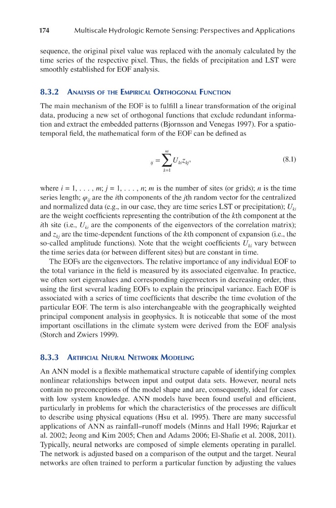
data, producing a new set of orthogonal functions that exclude redundant information and extract the embedded patterns (Bjornsson and Venegas 1997). For a spatiotemporal field, the mathematical form of the EOF can be defined as
ij
ki
k
m
kj
U z
=
=
∑
1
,
(8.1)
where i = 1, . . . , m; j = 1, . . . , n; m is the number of sites (or grids); n is the time
series length; φ ij are the ith components of the jth random vector for the centralized
and normalized data (e.g., in our case, they are time series LST or precipitation); U ki
are the weight coefficients representing the contribution of the kth component at the
ith site (i.e., U ki are the components of the eigenvectors of the correlation matrix);
and z kj are the time-dependent functions of the kth component of expansion (i.e., the
so-called amplitude functions). Note that the weight coefficients U ki vary between
the time series data (or between different sites) but are constant in time.
The EOFs are the eigenvectors. The relative importance of any individual EOF to
the total variance in the field is measured by its associated eigenvalue. In practice,
we often sort eigenvalues and corresponding eigenvectors in decreasing order, thus
using the first several leading EOFs to explain the principal variance. Each EOF is
associated with a series of time coefficients that describe the time evolution of the
particular EOF. The term is also interchangeable with the geographically weighted
principal component analysis in geophysics. It is noticeable that some of the most
important oscillations in the climate system were derived from the EOF analysis
(Storch and Zwiers 1999).
8.3.3 aRtificial neuRal netwoRk Modeling
An ANN model is a flexible mathematical structure capable of identifying complex
nonlinear relationships between input and output data sets. However, neural nets
contain no preconceptions of the model shape and are, consequently, ideal for cases
with low system knowledge. ANN models have been found useful and efficient,
particularly in problems for which the characteristics of the processes are difficult
to describe using physical equations (Hsu et al. 1995). There are many successful
applications of ANN as rainfall–runoff models (Minns and Hall 1996; Rajurkar et
al. 2002; Jeong and Kim 2005; Chen and Adams 2006; El-Shafie et al. 2008, 2011).
Typically, neural networks are composed of simple elements operating in parallel.
The network is adjusted based on a comparison of the output and the target. Neural
networks are often trained to perform a particular function by adjusting the values
Multiscale Hydrologic Remote Sensing: Perspectives and Applications
sequence, the original pixel value was replaced with the anomaly calculated by the
time series of the respective pixel. Thus, the fields of precipitation and LST were
smoothly established for EOF analysis.
8.3.2 analySiS of the eMPiRical oRthogonal function
The main mechanism of the EOF is to fulfill a linear transformation of the original
data, producing a new set of orthogonal functions that exclude redundant information and extract the embedded patterns (Bjornsson and Venegas 1997). For a spatiotemporal field, the mathematical form of the EOF can be defined as
ij
ki
k
m
kj
U z
=
=
∑
1
,
(8.1)
where i = 1, . . . , m; j = 1, . . . , n; m is the number of sites (or grids); n is the time
series length; φ ij are the ith components of the jth random vector for the centralized
and normalized data (e.g., in our case, they are time series LST or precipitation); U ki
are the weight coefficients representing the contribution of the kth component at the
ith site (i.e., U ki are the components of the eigenvectors of the correlation matrix);
and z kj are the time-dependent functions of the kth component of expansion (i.e., the
so-called amplitude functions). Note that the weight coefficients U ki vary between
the time series data (or between different sites) but are constant in time.
The EOFs are the eigenvectors. The relative importance of any individual EOF to
the total variance in the field is measured by its associated eigenvalue. In practice,
we often sort eigenvalues and corresponding eigenvectors in decreasing order, thus
using the first several leading EOFs to explain the principal variance. Each EOF is
associated with a series of time coefficients that describe the time evolution of the
particular EOF. The term is also interchangeable with the geographically weighted
principal component analysis in geophysics. It is noticeable that some of the most
important oscillations in the climate system were derived from the EOF analysis
(Storch and Zwiers 1999).
8.3.3 aRtificial neuRal netwoRk Modeling
An ANN model is a flexible mathematical structure capable of identifying complex
nonlinear relationships between input and output data sets. However, neural nets
contain no preconceptions of the model shape and are, consequently, ideal for cases
with low system knowledge. ANN models have been found useful and efficient,
particularly in problems for which the characteristics of the processes are difficult
to describe using physical equations (Hsu et al. 1995). There are many successful
applications of ANN as rainfall–runoff models (Minns and Hall 1996; Rajurkar et
al. 2002; Jeong and Kim 2005; Chen and Adams 2006; El-Shafie et al. 2008, 2011).
Typically, neural networks are composed of simple elements operating in parallel.
The network is adjusted based on a comparison of the output and the target. Neural
networks are often trained to perform a particular function by adjusting the values