

148
Multiscale Hydrologic Remote Sensing: Perspectives and Applications
where T s has the LST (in Kelvin), and a 6 and b 6 are the regression coefficients. For the
possible temperature range 0–70ºC, a 6 = –67.35535 and b 6 = 0.458608. Coefficients
C 6 and D 6 are defined for approximation expressed as follows:
C 6 = ε 6 τ 6
(7.7)
D 6 = (1 – τ 6 )[1 + (1 – ε 6 )τ 6 ],
(7.8)
where T a is the average effective mean atmospheric temperature (in Kelvin), τ 6 is the
atmospheric transmittance (in percent), and ε 6 is the ground emissivity (dimensionless). Therefore, if we know the parameter values of T a , τ 6 , and ε 6 , the LST of each
pixel can be derived using Equations 7.6 through 7.8. This study followed Equations
7.6 through 7.8 to derive the LST data.
7.2.6 calculationS of NDVI, ANDVI, MSAVI, and SAVI
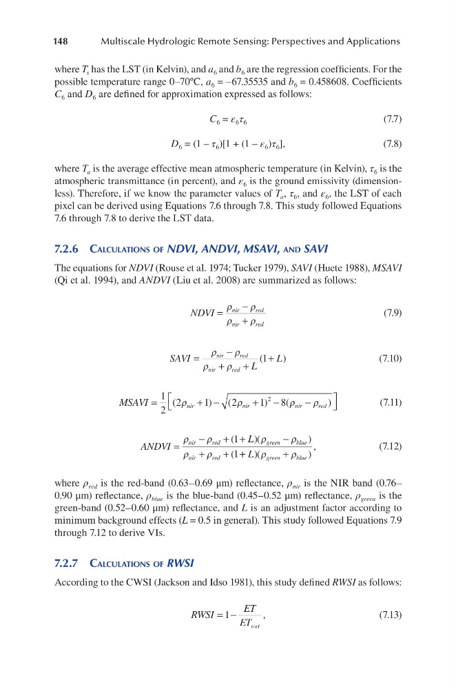
The equations for NDVI (Rouse et al. 1974; Tucker 1979), SAVI (Huete 1988), MSAVI
(Qi et al. 1994), and ANDVI (Liu et al. 2008) are summarized as follows:
NDVI
nir
red
nir
red
=
−
+
ρ
ρ
ρ
ρ
(7.9)
SAVI
L
L
nir
red
nir
red
=
−
+
+
+
ρ
ρ
ρ
ρ
(
)
1
(7.10)
MSAVI
nir
nir
nir
red
=
+ −
+ −
−
1
2
2
1
2
1
8
2
(
)
(
)
(
)
ρ
ρ
ρ
ρ
(7.11)
ANDVI
L
nir
red
green
blue
nir
red
=
−
+ +
−
+
+
ρ
ρ
ρ
ρ
ρ
ρ
(
)(
)
(
1
1 + +
+
L green
blue
)(
)
,
ρ
ρ
(7.12)
where ρ red is the red-band (0.63–0.69 μm) reflectance, ρ nir is the NIR band (0.76–
0.90 μm) reflectance, ρ blue is the blue-band (0.45–0.52 μm) reflectance, ρ green is the
green-band (0.52–0.60 μm) reflectance, and L is an adjustment factor according to
minimum background effects (L = 0.5 in general). This study followed Equations 7.9
through 7.12 to derive VIs.
7.2.7 calculationS of RWSI
According to the CWSI (Jackson and Idso 1981), this study defined RWSI as follows:
RWSI
ET
ET wet
= −
1
,
(7.13)
Multiscale Hydrologic Remote Sensing: Perspectives and Applications
where T s has the LST (in Kelvin), and a 6 and b 6 are the regression coefficients. For the
possible temperature range 0–70ºC, a 6 = –67.35535 and b 6 = 0.458608. Coefficients
C 6 and D 6 are defined for approximation expressed as follows:
C 6 = ε 6 τ 6
(7.7)
D 6 = (1 – τ 6 )[1 + (1 – ε 6 )τ 6 ],
(7.8)
where T a is the average effective mean atmospheric temperature (in Kelvin), τ 6 is the
atmospheric transmittance (in percent), and ε 6 is the ground emissivity (dimensionless). Therefore, if we know the parameter values of T a , τ 6 , and ε 6 , the LST of each
pixel can be derived using Equations 7.6 through 7.8. This study followed Equations
7.6 through 7.8 to derive the LST data.
7.2.6 calculationS of NDVI, ANDVI, MSAVI, and SAVI
The equations for NDVI (Rouse et al. 1974; Tucker 1979), SAVI (Huete 1988), MSAVI
(Qi et al. 1994), and ANDVI (Liu et al. 2008) are summarized as follows:
NDVI
nir
red
nir
red
=
−
+
ρ
ρ
ρ
ρ
(7.9)
SAVI
L
L
nir
red
nir
red
=
−
+
+
+
ρ
ρ
ρ
ρ
(
)
1
(7.10)
MSAVI
nir
nir
nir
red
=
+ −
+ −
−
1
2
2
1
2
1
8
2
(
)
(
)
(
)
ρ
ρ
ρ
ρ
(7.11)
ANDVI
L
nir
red
green
blue
nir
red
=
−
+ +
−
+
+
ρ
ρ
ρ
ρ
ρ
ρ
(
)(
)
(
1
1 + +
+
L green
blue
)(
)
,
ρ
ρ
(7.12)
where ρ red is the red-band (0.63–0.69 μm) reflectance, ρ nir is the NIR band (0.76–
0.90 μm) reflectance, ρ blue is the blue-band (0.45–0.52 μm) reflectance, ρ green is the
green-band (0.52–0.60 μm) reflectance, and L is an adjustment factor according to
minimum background effects (L = 0.5 in general). This study followed Equations 7.9
through 7.12 to derive VIs.
7.2.7 calculationS of RWSI
According to the CWSI (Jackson and Idso 1981), this study defined RWSI as follows:
RWSI
ET
ET wet
= −
1
,
(7.13)