

95
Thermal Radiation and Energy Closure Assessment
used as a first look (approximation) at the fluxes during the campaign. After the
campaign, the high-frequency data (20 Hz) were then processed in much greater
detail to arrive at the final turbulent fluxes for H and LE as described in the following section.
5.4 DATA TREATMENT
5.4.1 SPectRal analySiS
The turbulent process responsible for the exchange and transport of vertical fluxes
of heat and water vapor contains spectral information that describes the contribution of various frequencies to the observed velocity variances that are ultimately
component turbulent kinetic energy or covariances. Turbulent flows typically found
in the boundary layer (near a surface) are a superposition of many eddies varying in
scale and frequency. These eddies that are energy containing interact continuously
with the mean wind flow from where most of their energy is derived from and with
each other (i.e., eddy interaction at local and regional scales). To better understand
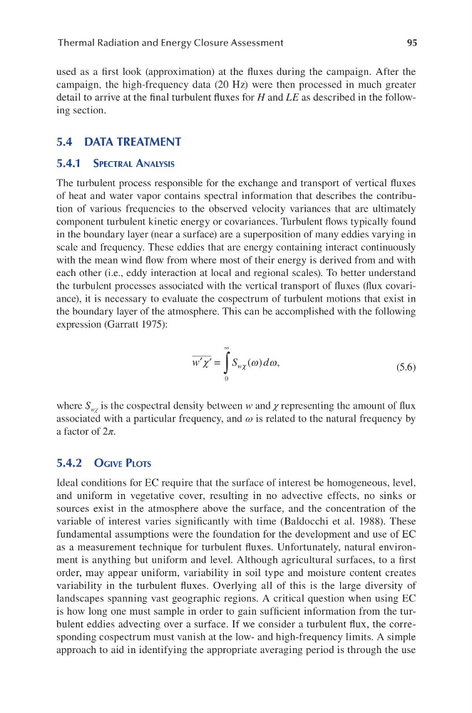
the turbulent processes associated with the vertical transport of fluxes (flux covariance), it is necessary to evaluate the cospectrum of turbulent motions that exist in
the boundary layer of the atmosphere. This can be accomplished with the following
expression (Garratt 1975):
′ ′
∞
∫
w
d
w
χ
χ
= S ( )
ω ω,
0
(5.6)
where S wχ is the cospectral density between w and χ representing the amount of flux
associated with a particular frequency, and ω is related to the natural frequency by
a factor of 2π.
5.4.2 ogive PlotS
Ideal conditions for EC require that the surface of interest be homogeneous, level,
and uniform in vegetative cover, resulting in no advective effects, no sinks or
sources exist in the atmosphere above the surface, and the concentration of the
variable of interest varies significantly with time (Baldocchi et al. 1988). These
fundamental assumptions were the foundation for the development and use of EC
as a measurement technique for turbulent fluxes. Unfortunately, natural environment is anything but uniform and level. Although agricultural surfaces, to a first
order, may appear uniform, variability in soil type and moisture content creates
variability in the turbulent fluxes. Overlying all of this is the large diversity of
landscapes spanning vast geographic regions. A critical question when using EC
is how long one must sample in order to gain sufficient information from the turbulent eddies advecting over a surface. If we consider a turbulent flux, the corresponding cospectrum must vanish at the low- and high-frequency limits. A simple
approach to aid in identifying the appropriate averaging period is through the use
Thermal Radiation and Energy Closure Assessment
used as a first look (approximation) at the fluxes during the campaign. After the
campaign, the high-frequency data (20 Hz) were then processed in much greater
detail to arrive at the final turbulent fluxes for H and LE as described in the following section.
5.4 DATA TREATMENT
5.4.1 SPectRal analySiS
The turbulent process responsible for the exchange and transport of vertical fluxes
of heat and water vapor contains spectral information that describes the contribution of various frequencies to the observed velocity variances that are ultimately
component turbulent kinetic energy or covariances. Turbulent flows typically found
in the boundary layer (near a surface) are a superposition of many eddies varying in
scale and frequency. These eddies that are energy containing interact continuously
with the mean wind flow from where most of their energy is derived from and with
each other (i.e., eddy interaction at local and regional scales). To better understand
the turbulent processes associated with the vertical transport of fluxes (flux covariance), it is necessary to evaluate the cospectrum of turbulent motions that exist in
the boundary layer of the atmosphere. This can be accomplished with the following
expression (Garratt 1975):
′ ′
∞
∫
w
d
w
χ
χ
= S ( )
ω ω,
0
(5.6)
where S wχ is the cospectral density between w and χ representing the amount of flux
associated with a particular frequency, and ω is related to the natural frequency by
a factor of 2π.
5.4.2 ogive PlotS
Ideal conditions for EC require that the surface of interest be homogeneous, level,
and uniform in vegetative cover, resulting in no advective effects, no sinks or
sources exist in the atmosphere above the surface, and the concentration of the
variable of interest varies significantly with time (Baldocchi et al. 1988). These
fundamental assumptions were the foundation for the development and use of EC
as a measurement technique for turbulent fluxes. Unfortunately, natural environment is anything but uniform and level. Although agricultural surfaces, to a first
order, may appear uniform, variability in soil type and moisture content creates
variability in the turbulent fluxes. Overlying all of this is the large diversity of
landscapes spanning vast geographic regions. A critical question when using EC
is how long one must sample in order to gain sufficient information from the turbulent eddies advecting over a surface. If we consider a turbulent flux, the corresponding cospectrum must vanish at the low- and high-frequency limits. A simple
approach to aid in identifying the appropriate averaging period is through the use