

96
Multiscale Hydrologic Remote Sensing: Perspectives and Applications
of the cospectrum. For any covariance, it is mathematically a cumulative cospectrum expressed simply as
Γ w
w
w
Co x dx
χ
χ
λ
χ
( )
1
( ) ,
= ′ ′
∞
∫
0
(5.7)
where Γ wχ is the cumulative cospectrum energy, and Co wχ is the cospectrum of w and
χ. The graph of Γ wχ is often called an “ogive” (oh-jive) curve (Desjardins et al. 1989;
Friehe et al. 1991; Lambert et al. 1999). The resulting ogive curve is the integration
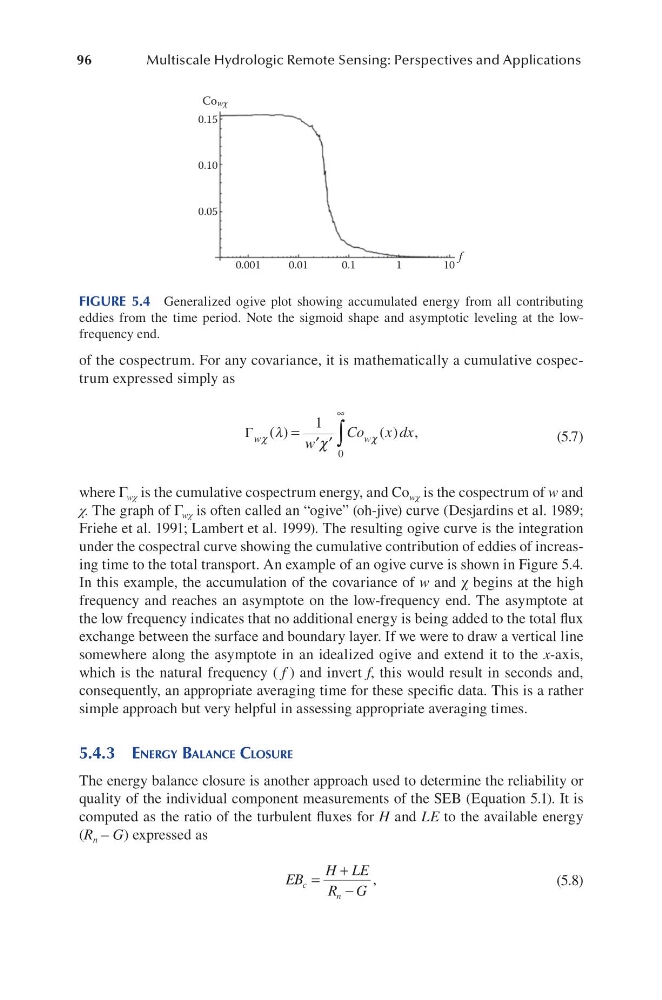
under the cospectral curve showing the cumulative contribution of eddies of increasing time to the total transport. An example of an ogive curve is shown in Figure 5.4.
In this example, the accumulation of the covariance of w and χ begins at the high
frequency and reaches an asymptote on the low-frequency end. The asymptote at
the low frequency indicates that no additional energy is being added to the total flux
exchange between the surface and boundary layer. If we were to draw a vertical line
somewhere along the asymptote in an idealized ogive and extend it to the x-axis,
which is the natural frequency ( f ) and invert f, this would result in seconds and,
consequently, an appropriate averaging time for these specific data. This is a rather
simple approach but very helpful in assessing appropriate averaging times.
5.4.3 eneRgy Balance cloSuRe
The energy balance closure is another approach used to determine the reliability or
quality of the individual component measurements of the SEB (Equation 5.1). It is
computed as the ratio of the turbulent fluxes for H and LE to the available energy
(R n – G) expressed as
EB
H LE
R G
c
n
=
+
−
,
(5.8)
0.15
0.10
0.05
0.001
0.01
0.1
1
10
f
Cowχ
FIGURE 5.4 Generalized ogive plot showing accumulated energy from all contributing
eddies from the time period. Note the sigmoid shape and asymptotic leveling at the lowfrequency end.
Multiscale Hydrologic Remote Sensing: Perspectives and Applications
of the cospectrum. For any covariance, it is mathematically a cumulative cospectrum expressed simply as
Γ w
w
w
Co x dx
χ
χ
λ
χ
( )
1
( ) ,
= ′ ′
∞
∫
0
(5.7)
where Γ wχ is the cumulative cospectrum energy, and Co wχ is the cospectrum of w and
χ. The graph of Γ wχ is often called an “ogive” (oh-jive) curve (Desjardins et al. 1989;
Friehe et al. 1991; Lambert et al. 1999). The resulting ogive curve is the integration
under the cospectral curve showing the cumulative contribution of eddies of increasing time to the total transport. An example of an ogive curve is shown in Figure 5.4.
In this example, the accumulation of the covariance of w and χ begins at the high
frequency and reaches an asymptote on the low-frequency end. The asymptote at
the low frequency indicates that no additional energy is being added to the total flux
exchange between the surface and boundary layer. If we were to draw a vertical line
somewhere along the asymptote in an idealized ogive and extend it to the x-axis,
which is the natural frequency ( f ) and invert f, this would result in seconds and,
consequently, an appropriate averaging time for these specific data. This is a rather
simple approach but very helpful in assessing appropriate averaging times.
5.4.3 eneRgy Balance cloSuRe
The energy balance closure is another approach used to determine the reliability or
quality of the individual component measurements of the SEB (Equation 5.1). It is
computed as the ratio of the turbulent fluxes for H and LE to the available energy
(R n – G) expressed as
EB
H LE
R G
c
n
=
+
−
,
(5.8)
0.15
0.10
0.05
0.001
0.01
0.1
1
10
f
Cowχ
FIGURE 5.4 Generalized ogive plot showing accumulated energy from all contributing
eddies from the time period. Note the sigmoid shape and asymptotic leveling at the lowfrequency end.