

543
• Both models contain the possibility to simulate
bioirrigation; STEADYSED1 generally treats
bioirrigation and bioturbation with much more
thoroughness and reliability.
• STEADYSED1 is quite limited as far as its
chemical processes are concerned (absence of
real activities in the pore water, and hence only
apparent equilibrium constants, complex
species are not included). However, it contains
all the essential processes currently known.
CoTReM is much more flexible owing to the
utilization of PHREEQC (Parkhurst 1995) as a
subroutine, yet it requires proportionally more
information.
• The model CoTReM works with Fick’s Second
Law of Diffusion and thus permits the
calculation of any possible, especially nonsteady state situations. STEADYSED1 can
only be applied to calculate steady state
situations which accordingly demand the
existence of steady state boundary conditions.
15.4 Bioturbation and Bioirrigation
in Combined Models
Bioturbation is normally modeled by applying a
bio-diffusion coefficient to the pore water
fraction and the solid phase. This means that a
bio-diffusion in the solid phase will be simulated with the same model concept which is
applied in the form of Fick’s laws to the dissolved constituents in pore water. Under the
assumption of a given steady state (e.g.
STEADYSED1), this requires that a sufficient
length of time is studied which allows the
macroorganisms contributing to bioturbation to
display activity all over and as many times as
appears necessary. Only then will each part of
the solid phase be turned over often enough in
the statistical balance, hence providing a
workable model concept. As for cases of nonsteady state and short observation periods the
model concept actually cannot be considered
as valid.
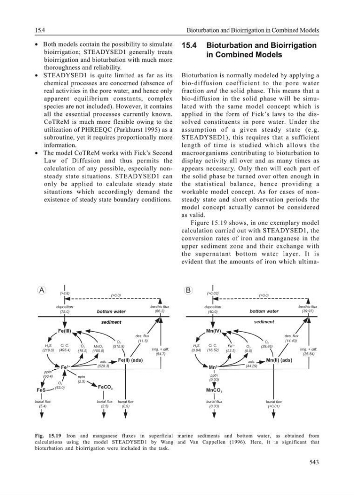
Figure 15.19 shows, in one exemplary model
calculation carried out with STEADYSED1, the
conversion rates of iron and manganese in the
upper sediment zone and their exchange with
the supernatant bottom water layer. It is
evident that the amounts of iron which ultima(>8.8)
(75.0)
deposition
(>0.0)
(66.2)
benthic flux
(11.5)
des. flux
(515.9)
O 2
(219.0)
H 2 S
(495.4)
O. C.
(18.5)
O 2
(105.0)
MnO 2
(528.3)
ads.
(68.4)
pptn
(2.5)
pptn
(63.0)
O 2
(5.4)
burial flux
(2.5)
burial flux
(0.9)
burial flux
(54.7)
irrig. + diff.
Fe(III)
Fe
2+
Fe(II) (ads)
FeCO 3
FeS
(>0.03)
(40.0)
deposition
(>0.0)
(39.97)
benthic flux
(14.43)
des. flux
(29.86)
O 2
(0.84)
H 2 S
(16.52)
O. C.
(52.5)
Fe 2+
(0.0)
O 2
(44.29)
ads.
(0.03)
pptn
(0.03)
burial flux
(<0.01)
burial flux
(25.54)
irrig. + diff.
Mn(IV)
Mn
2+
Mn(II) (ads)
MnCO 3
bottom water
sediment
bottom water
sediment
A
B
Fig. 15.19 Iron and manganese fluxes in superficial marine sediments and bottom water, as obtained from
calculations using the model STEADYSED1 by Wang and Van Cappellen (1996). Here, it is significant that
bioturbation and bioirrigation were included in the task.
15.4
Bioturbation and Bioirrigation in Combined Models
• Both models contain the possibility to simulate
bioirrigation; STEADYSED1 generally treats
bioirrigation and bioturbation with much more
thoroughness and reliability.
• STEADYSED1 is quite limited as far as its
chemical processes are concerned (absence of
real activities in the pore water, and hence only
apparent equilibrium constants, complex
species are not included). However, it contains
all the essential processes currently known.
CoTReM is much more flexible owing to the
utilization of PHREEQC (Parkhurst 1995) as a
subroutine, yet it requires proportionally more
information.
• The model CoTReM works with Fick’s Second
Law of Diffusion and thus permits the
calculation of any possible, especially nonsteady state situations. STEADYSED1 can
only be applied to calculate steady state
situations which accordingly demand the
existence of steady state boundary conditions.
15.4 Bioturbation and Bioirrigation
in Combined Models
Bioturbation is normally modeled by applying a
bio-diffusion coefficient to the pore water
fraction and the solid phase. This means that a
bio-diffusion in the solid phase will be simulated with the same model concept which is
applied in the form of Fick’s laws to the dissolved constituents in pore water. Under the
assumption of a given steady state (e.g.
STEADYSED1), this requires that a sufficient
length of time is studied which allows the
macroorganisms contributing to bioturbation to
display activity all over and as many times as
appears necessary. Only then will each part of
the solid phase be turned over often enough in
the statistical balance, hence providing a
workable model concept. As for cases of nonsteady state and short observation periods the
model concept actually cannot be considered
as valid.
Figure 15.19 shows, in one exemplary model
calculation carried out with STEADYSED1, the
conversion rates of iron and manganese in the
upper sediment zone and their exchange with
the supernatant bottom water layer. It is
evident that the amounts of iron which ultima(>8.8)
(75.0)
deposition
(>0.0)
(66.2)
benthic flux
(11.5)
des. flux
(515.9)
O 2
(219.0)
H 2 S
(495.4)
O. C.
(18.5)
O 2
(105.0)
MnO 2
(528.3)
ads.
(68.4)
pptn
(2.5)
pptn
(63.0)
O 2
(5.4)
burial flux
(2.5)
burial flux
(0.9)
burial flux
(54.7)
irrig. + diff.
Fe(III)
Fe
2+
Fe(II) (ads)
FeCO 3
FeS
(>0.03)
(40.0)
deposition
(>0.0)
(39.97)
benthic flux
(14.43)
des. flux
(29.86)
O 2
(0.84)
H 2 S
(16.52)
O. C.
(52.5)
Fe 2+
(0.0)
O 2
(44.29)
ads.
(0.03)
pptn
(0.03)
burial flux
(<0.01)
burial flux
(25.54)
irrig. + diff.
Mn(IV)
Mn
2+
Mn(II) (ads)
MnCO 3
bottom water
sediment
bottom water
sediment
A
B
Fig. 15.19 Iron and manganese fluxes in superficial marine sediments and bottom water, as obtained from
calculations using the model STEADYSED1 by Wang and Van Cappellen (1996). Here, it is significant that
bioturbation and bioirrigation were included in the task.
15.4
Bioturbation and Bioirrigation in Combined Models