

15 Conceptual Models and Computer Models
544
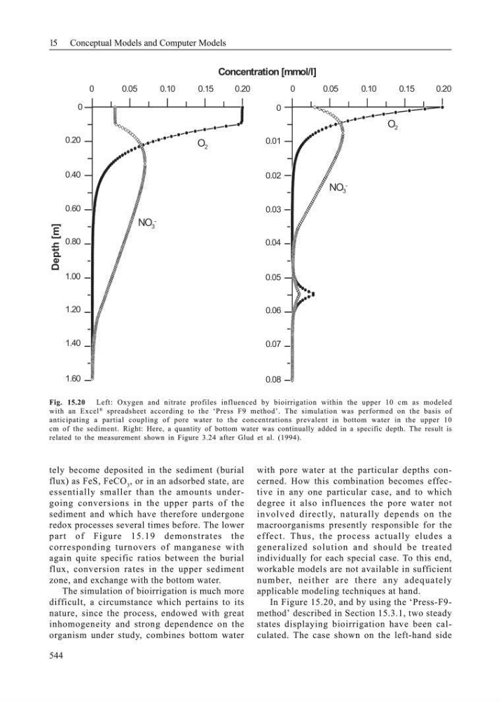
Fig. 15.20
Left: Oxygen and nitrate profiles influenced by bioirrigation within the upper 10 cm as modeled
with an Excel
® spreadsheet according to the ‘Press F9 method’. The simulation was performed on the basis of
anticipating a partial coupling of pore water to the concentrations prevalent in bottom water in the upper 10
cm of the sediment. Right: Here, a quantity of bottom water was continually added in a specific depth. The result is
related to the measurement shown in Figure 3.24 after Glud et al. (1994).
1.60
1.40
1.20
1.00
0.80
0.60
0.40
0.20
0
Depth [m]
0.05
0.10
0.15
0.20
0
0.08
0.07
0.06
0.05
0.04
0.03
0.02
0.01
0
0.05
0.10
0.15
0.20
0
Concentration [mmol/l]
O 2
O 2
NO 3
-
NO 3
-
tely become deposited in the sediment (burial
flux) as FeS, FeCO 3 , or in an adsorbed state, are
essentially smaller than the amounts undergoing conversions in the upper parts of the
sediment and which have therefore undergone
redox processes several times before. The lower
part of Figure 15.19 demonstrates the
corresponding turnovers of manganese with
again quite specific ratios between the burial
flux, conversion rates in the upper sediment
zone, and exchange with the bottom water.
The simulation of bioirrigation is much more
difficult, a circumstance which pertains to its
nature, since the process, endowed with great
inhomogeneity and strong dependence on the
organism under study, combines bottom water
with pore water at the particular depths concerned. How this combination becomes effective in any one particular case, and to which
degree it also influences the pore water not
involved directly, naturally depends on the
macroorganisms presently responsible for the
effect. Thus, the process actually eludes a
generalized solution and should be treated
individually for each special case. To this end,
workable models are not available in sufficient
number, neither are there any adequately
applicable modeling techniques at hand.
In Figure 15.20, and by using the ‘Press-F9method’ described in Section 15.3.1, two steady
states displaying bioirrigation have been calculated. The case shown on the left-hand side
544
Fig. 15.20
Left: Oxygen and nitrate profiles influenced by bioirrigation within the upper 10 cm as modeled
with an Excel
® spreadsheet according to the ‘Press F9 method’. The simulation was performed on the basis of
anticipating a partial coupling of pore water to the concentrations prevalent in bottom water in the upper 10
cm of the sediment. Right: Here, a quantity of bottom water was continually added in a specific depth. The result is
related to the measurement shown in Figure 3.24 after Glud et al. (1994).
1.60
1.40
1.20
1.00
0.80
0.60
0.40
0.20
0
Depth [m]
0.05
0.10
0.15
0.20
0
0.08
0.07
0.06
0.05
0.04
0.03
0.02
0.01
0
0.05
0.10
0.15
0.20
0
Concentration [mmol/l]
O 2
O 2
NO 3
-
NO 3
-
tely become deposited in the sediment (burial
flux) as FeS, FeCO 3 , or in an adsorbed state, are
essentially smaller than the amounts undergoing conversions in the upper parts of the
sediment and which have therefore undergone
redox processes several times before. The lower
part of Figure 15.19 demonstrates the
corresponding turnovers of manganese with
again quite specific ratios between the burial
flux, conversion rates in the upper sediment
zone, and exchange with the bottom water.
The simulation of bioirrigation is much more
difficult, a circumstance which pertains to its
nature, since the process, endowed with great
inhomogeneity and strong dependence on the
organism under study, combines bottom water
with pore water at the particular depths concerned. How this combination becomes effective in any one particular case, and to which
degree it also influences the pore water not
involved directly, naturally depends on the
macroorganisms presently responsible for the
effect. Thus, the process actually eludes a
generalized solution and should be treated
individually for each special case. To this end,
workable models are not available in sufficient
number, neither are there any adequately
applicable modeling techniques at hand.
In Figure 15.20, and by using the ‘Press-F9method’ described in Section 15.3.1, two steady
states displaying bioirrigation have been calculated. The case shown on the left-hand side