

531
whereby distinctly shorter time-steps may also be
used without causing any problem.
sed
D
x
t
⋅
∆
≤
∆
2
2
15.9
The explicit solution can be realized quite reasonably with an Excel
®
worksheet in the sense of the
‚Press-F9-Method’ (Section 15.3.1). However, in
most cases a program written in a higher programming language will be applied, since this type
of modeling is made because one desires to include more complex (bio)geochemical reactions.
And sooner or later the limits of modeling are
reached when an Excel
®
worksheet is used.
An easy to handle and rather generally designed computer model written in FORTRAN
(EXPLICIT.FOR) can be downloaded on the
internet at:
http://www.geochemie.uni-bremen.de/downloads/
along with brief user instructions written in English and data sets pertaining to several examples.
The following examples (Example 1 and 2)
were calculated using this program. Subsequent
examples (Examples 3 and 4) reveal how an
explicit solution was realized with an Excel
®
worksheet in the sense of the ‚Press-F9-Method’
(Section 15.3.1). Downloads of these worksheets
are also available at the above mentioned internet address.
Example 1: Non-steady state development of an
oxygen profile
An oxygen concentration profile such as the one
which has been measured in situ (Fig. 3.5) or
modeled (Fig. 15.5) is mostly interpreted in terms
of a stationary condition (steady state) resulting
from the consumption of oxygen in the sediment
and its resupply by means of diffusion. Its consumption in the sediment is due to the oxidation
of organic matter and other redox processes, such
as the re-oxidation of divalent manganese. But
how long does it take until such a stationary
condition is reached ?
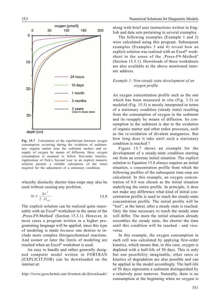
Figure 15.7 shows an example for the
development of a steady-state condition starting
out from an extreme initial situation. The explicit
solution to Equation 15.8 always requires an initial
situation, a concentration profile from which the
following profiles of the subsequent time-step are
calculated. In this example, an oxygen concentration of 0.0 was chosen as the initial situation
underlying the entire profile. In principle, it does
not make any difference what kind of initial concentration profile is used to reach the steady-state
concentration profile. The initial profile will be
“lost”, at the latest, after a steady state is reached.
Only the time necessary to reach the steady state
will differ. The more the initial situation already
resembles the steady state, the shorter the time
until this condition will be reached - and viceversa.
In this example, the oxygen consumption in
each cell was calculated by applying first-order
kinetics, which means that, in this case, oxygen is
depleted with a half-life of 50 days. This is only
but one possibility imaginable, other rates or
kinetics of degradation are also possible and can
be applied in the model accordingly. The half-life
of 50 days represents a sediment distinguished by
a relatively poor turnover. Naturally, there is no
consumption at the beginning when no oxygen is
15.3
Numerical Solutions for Diagenetic Models
Fig. 15.7 Calculation of the equilibrium between oxygen
consumption occurring during the oxidation of sedimentary organic matter near the sediment surface and resupply of oxygen by means of diffusion. Here, oxygen
consumption is assumed to follow first-order kinetics.
Application of Fick’s Second Law in an explicit numeric
solution permits a reliable calculation of the times
required for the adjustment of a stationary condition.
whereby distinctly shorter time-steps may also be
used without causing any problem.
sed
D
x
t
⋅
∆
≤
∆
2
2
15.9
The explicit solution can be realized quite reasonably with an Excel
®
worksheet in the sense of the
‚Press-F9-Method’ (Section 15.3.1). However, in
most cases a program written in a higher programming language will be applied, since this type
of modeling is made because one desires to include more complex (bio)geochemical reactions.
And sooner or later the limits of modeling are
reached when an Excel
®
worksheet is used.
An easy to handle and rather generally designed computer model written in FORTRAN
(EXPLICIT.FOR) can be downloaded on the
internet at:
http://www.geochemie.uni-bremen.de/downloads/
along with brief user instructions written in English and data sets pertaining to several examples.
The following examples (Example 1 and 2)
were calculated using this program. Subsequent
examples (Examples 3 and 4) reveal how an
explicit solution was realized with an Excel
®
worksheet in the sense of the ‚Press-F9-Method’
(Section 15.3.1). Downloads of these worksheets
are also available at the above mentioned internet address.
Example 1: Non-steady state development of an
oxygen profile
An oxygen concentration profile such as the one
which has been measured in situ (Fig. 3.5) or
modeled (Fig. 15.5) is mostly interpreted in terms
of a stationary condition (steady state) resulting
from the consumption of oxygen in the sediment
and its resupply by means of diffusion. Its consumption in the sediment is due to the oxidation
of organic matter and other redox processes, such
as the re-oxidation of divalent manganese. But
how long does it take until such a stationary
condition is reached ?
Figure 15.7 shows an example for the
development of a steady-state condition starting
out from an extreme initial situation. The explicit
solution to Equation 15.8 always requires an initial
situation, a concentration profile from which the
following profiles of the subsequent time-step are
calculated. In this example, an oxygen concentration of 0.0 was chosen as the initial situation
underlying the entire profile. In principle, it does
not make any difference what kind of initial concentration profile is used to reach the steady-state
concentration profile. The initial profile will be
“lost”, at the latest, after a steady state is reached.
Only the time necessary to reach the steady state
will differ. The more the initial situation already
resembles the steady state, the shorter the time
until this condition will be reached - and viceversa.
In this example, the oxygen consumption in
each cell was calculated by applying first-order
kinetics, which means that, in this case, oxygen is
depleted with a half-life of 50 days. This is only
but one possibility imaginable, other rates or
kinetics of degradation are also possible and can
be applied in the model accordingly. The half-life
of 50 days represents a sediment distinguished by
a relatively poor turnover. Naturally, there is no
consumption at the beginning when no oxygen is
15.3
Numerical Solutions for Diagenetic Models
Fig. 15.7 Calculation of the equilibrium between oxygen
consumption occurring during the oxidation of sedimentary organic matter near the sediment surface and resupply of oxygen by means of diffusion. Here, oxygen
consumption is assumed to follow first-order kinetics.
Application of Fick’s Second Law in an explicit numeric
solution permits a reliable calculation of the times
required for the adjustment of a stationary condition.