

15 Conceptual Models and Computer Models
530
tion that cannot be applied for mathematical
reasons in this regard. Then physical transport is
calculated once again on the basis of the concentrations thus calculated, followed by a
subsequent calculation of the reactions etc. This
procedure is referred to as the “Two-Step
Method” or “Operator Splitting”. It will be
discussed more thoroughly in the following. As
much as we know, this method has been applied
for the first time by Schulz and Readon (1983).
Here, only the simplest form of such a modeling
process, the so-called explicit solution, will be
presented for introductory purposes. It rapidly
illustrates the principle of the Two-Step Method
and suffices completely to achieve adequate
modeling results in most practical situations.
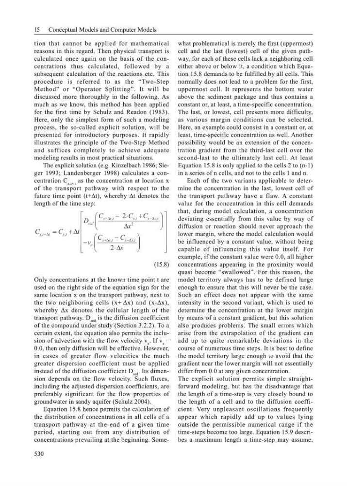
The explicit solution (e.g. Kinzelbach 1986; Sieger 1993; Landenberger 1998) calculates a concentration C x,t+ t as the concentration at location x
of the transport pathway with respect to the
future time point (t+∆t), whereby ∆t denotes the
length of the time step:
⎥
⎥
⎥
⎥
⎥
⎦
⎤
⎢
⎢
⎢
⎢
⎢
⎣
⎡
⎟ ⎟
⎠
⎞
⎜ ⎜
⎝
⎛
∆
⋅
−
−
⎟ ⎟
⎠
⎞
⎜ ⎜
⎝
⎛
∆
+
⋅
−
∆
+
=
∆
−
∆
+
∆
−
∆
+
∆
+
x
C
C
v
x
C
C
C
D
t
C
C
t
x
x
t
x
x
a
t
x
x
t
x
t
x
x
sed
t
x
t
t
x
2
2
,
,
2
,
,
,
,
,
(15.8)
Only concentrations at the known time point t are
used on the right side of the equation sign for the
same location x on the transport pathway, next to
the two neighboring cells (x+ ∆x) and (x-∆x),
whereby ∆x denotes the cellular length of the
transport pathway. D sed is the diffusion coefficient
of the compound under study (Section 3.2.2). To a
certain extent, the equation also permits the inclusion of advection with the flow velocity v a . If v a =
0.0, then only diffusion will be effective. However,
in cases of greater flow velocities the much
greater dispersion coefficient must be applied
instead of the diffusion coefficient D sed . Its dimension depends on the flow velocity. Such fluxes,
including the adjusted dispersion coefficients, are
preferably significant for the flow properties of
groundwater in sandy aquifer (Schulz 2004).
Equation 15.8 hence permits the calculation of
the distribution of concentrations in all cells of a
transport pathway at the end of a given time
period, starting out from any distribution of
concentrations prevailing at the beginning. Somewhat problematical is merely the first (uppermost)
cell and the last (lowest) cell of the given pathway, for each of these cells lack a neighboring cell
either above or below it, a condition which Equation 15.8 demands to be fulfilled by all cells. This
normally does not lead to a problem for the first,
uppermost cell. It represents the bottom water
above the sediment package and thus contains a
constant or, at least, a time-specific concentration.
The last, or lowest, cell presents more difficulty,
as various margin conditions can be selected.
Here, an example could consist in a constant or, at
least, time-specific concentration as well. Another
possibility would be an extension of the concentration gradient from the third-last cell over the
second-last to the ultimately last cell. At least
Equation 15.8 is only applied to the cells 2 to (n-1)
in a series of n cells, and not to the cells 1 and n.
Each of the two variants applicable to determine the concentration in the last, lowest cell of
the transport pathway have a flaw. A constant
value for the concentration in this cell demands
that, during model calculation, a concentration
deviating essentially from this value by way of
diffusion or reaction should never approach the
lower margin, where the model calculation would
be influenced by a constant value, without being
capable of influencing this value itself. For
example, if the constant value were 0.0, all higher
concentrations appearing in the proximity would
quasi become “swallowed”. For this reason, the
model territory always has to be defined large
enough to ensure that this will never be the case.
Such an effect does not appear with the same
intensity in the second variant, which is used to
determine the concentration at the lower margin
by means of a constant gradient, but this solution
also produces problems. The small errors which
arise from the extrapolation of the gradient can
add up to quite remarkable deviations in the
course of numerous time steps. It is best to define
the model territory large enough to avoid that the
gradient near the lower margin will not essentially
differ from 0.0 at any given concentration.
The explicit solution permits simple straightforward modeling, but has the disadvantage that
the length of a time-step is very closely bound to
the length of a cell and to the diffusion coefficient. Very unpleasant oscillations frequently
appear which rapidly add up to values lying
outside the permissible numerical range if the
time-steps become too large. Equation 15.9 describes a maximum length a time-step may assume,
530
tion that cannot be applied for mathematical
reasons in this regard. Then physical transport is
calculated once again on the basis of the concentrations thus calculated, followed by a
subsequent calculation of the reactions etc. This
procedure is referred to as the “Two-Step
Method” or “Operator Splitting”. It will be
discussed more thoroughly in the following. As
much as we know, this method has been applied
for the first time by Schulz and Readon (1983).
Here, only the simplest form of such a modeling
process, the so-called explicit solution, will be
presented for introductory purposes. It rapidly
illustrates the principle of the Two-Step Method
and suffices completely to achieve adequate
modeling results in most practical situations.
The explicit solution (e.g. Kinzelbach 1986; Sieger 1993; Landenberger 1998) calculates a concentration C x,t+ t as the concentration at location x
of the transport pathway with respect to the
future time point (t+∆t), whereby ∆t denotes the
length of the time step:
⎥
⎥
⎥
⎥
⎥
⎦
⎤
⎢
⎢
⎢
⎢
⎢
⎣
⎡
⎟ ⎟
⎠
⎞
⎜ ⎜
⎝
⎛
∆
⋅
−
−
⎟ ⎟
⎠
⎞
⎜ ⎜
⎝
⎛
∆
+
⋅
−
∆
+
=
∆
−
∆
+
∆
−
∆
+
∆
+
x
C
C
v
x
C
C
C
D
t
C
C
t
x
x
t
x
x
a
t
x
x
t
x
t
x
x
sed
t
x
t
t
x
2
2
,
,
2
,
,
,
,
,
(15.8)
Only concentrations at the known time point t are
used on the right side of the equation sign for the
same location x on the transport pathway, next to
the two neighboring cells (x+ ∆x) and (x-∆x),
whereby ∆x denotes the cellular length of the
transport pathway. D sed is the diffusion coefficient
of the compound under study (Section 3.2.2). To a
certain extent, the equation also permits the inclusion of advection with the flow velocity v a . If v a =
0.0, then only diffusion will be effective. However,
in cases of greater flow velocities the much
greater dispersion coefficient must be applied
instead of the diffusion coefficient D sed . Its dimension depends on the flow velocity. Such fluxes,
including the adjusted dispersion coefficients, are
preferably significant for the flow properties of
groundwater in sandy aquifer (Schulz 2004).
Equation 15.8 hence permits the calculation of
the distribution of concentrations in all cells of a
transport pathway at the end of a given time
period, starting out from any distribution of
concentrations prevailing at the beginning. Somewhat problematical is merely the first (uppermost)
cell and the last (lowest) cell of the given pathway, for each of these cells lack a neighboring cell
either above or below it, a condition which Equation 15.8 demands to be fulfilled by all cells. This
normally does not lead to a problem for the first,
uppermost cell. It represents the bottom water
above the sediment package and thus contains a
constant or, at least, a time-specific concentration.
The last, or lowest, cell presents more difficulty,
as various margin conditions can be selected.
Here, an example could consist in a constant or, at
least, time-specific concentration as well. Another
possibility would be an extension of the concentration gradient from the third-last cell over the
second-last to the ultimately last cell. At least
Equation 15.8 is only applied to the cells 2 to (n-1)
in a series of n cells, and not to the cells 1 and n.
Each of the two variants applicable to determine the concentration in the last, lowest cell of
the transport pathway have a flaw. A constant
value for the concentration in this cell demands
that, during model calculation, a concentration
deviating essentially from this value by way of
diffusion or reaction should never approach the
lower margin, where the model calculation would
be influenced by a constant value, without being
capable of influencing this value itself. For
example, if the constant value were 0.0, all higher
concentrations appearing in the proximity would
quasi become “swallowed”. For this reason, the
model territory always has to be defined large
enough to ensure that this will never be the case.
Such an effect does not appear with the same
intensity in the second variant, which is used to
determine the concentration at the lower margin
by means of a constant gradient, but this solution
also produces problems. The small errors which
arise from the extrapolation of the gradient can
add up to quite remarkable deviations in the
course of numerous time steps. It is best to define
the model territory large enough to avoid that the
gradient near the lower margin will not essentially
differ from 0.0 at any given concentration.
The explicit solution permits simple straightforward modeling, but has the disadvantage that
the length of a time-step is very closely bound to
the length of a cell and to the diffusion coefficient. Very unpleasant oscillations frequently
appear which rapidly add up to values lying
outside the permissible numerical range if the
time-steps become too large. Equation 15.9 describes a maximum length a time-step may assume,