

529
15.3
Numerical Solutions for Diagenetic Models
0
2
4
6
8
10
12
14
0
5
1 0
15
20
0
5 10 15 20 25 30
0
5 10 15 20 25 30
Depth [m]
CH 4 [mmol/l]
SO 4 [mmol/l]
CH 4 , SO 4 [mmol/l]
GeoB 3718
core catcher
directly after
coring
m
o d e l s u l f a t e
m
o d e l m e t h a n e
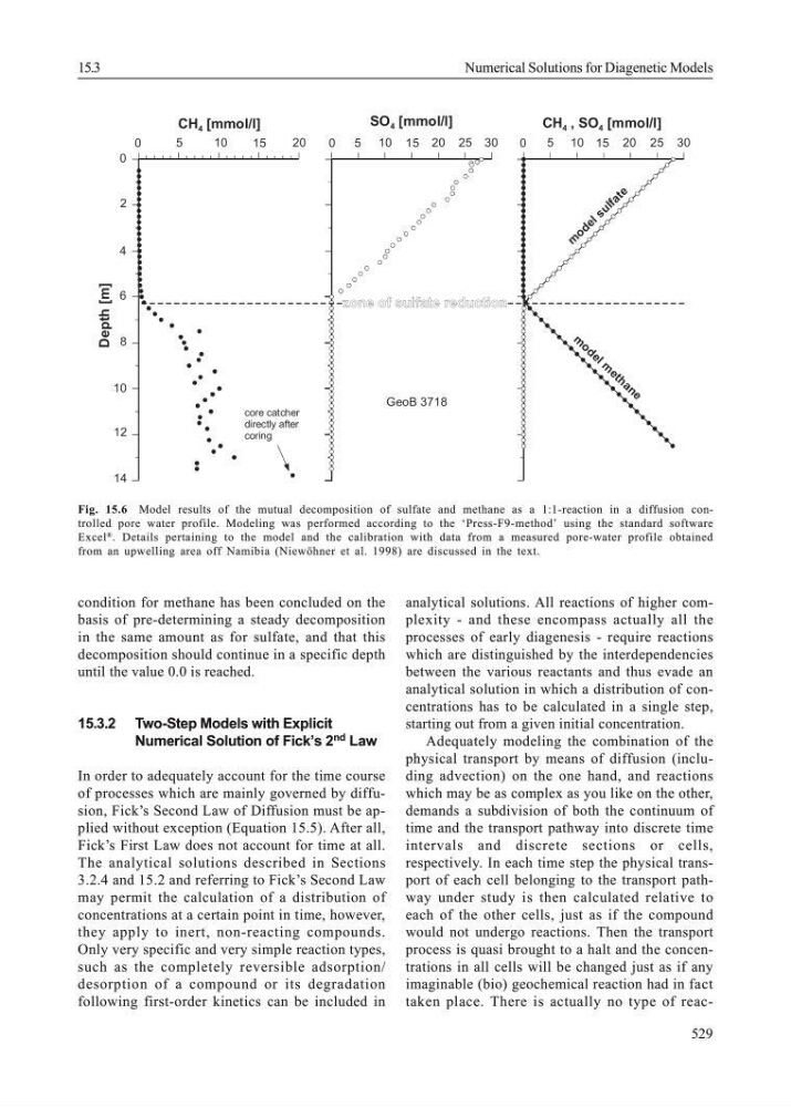
Fig. 15.6 Model results of the mutual decomposition of sulfate and methane as a 1:1-reaction in a diffusion controlled pore water profile. Modeling was performed according to the ‘Press-F9-method’ using the standard software
Excel
® . Details pertaining to the model and the calibration with data from a measured pore-water profile obtained
from an upwelling area off Namibia (Niewöhner et al. 1998) are discussed in the text.
condition for methane has been concluded on the
basis of pre-determining a steady decomposition
in the same amount as for sulfate, and that this
decomposition should continue in a specific depth
until the value 0.0 is reached.
15.3.2 Two-Step Models with Explicit
Numerical Solution of Fick’s 2 nd Law
In order to adequately account for the time course
of processes which are mainly governed by diffusion, Fick’s Second Law of Diffusion must be applied without exception (Equation 15.5). After all,
Fick’s First Law does not account for time at all.
The analytical solutions described in Sections
3.2.4 and 15.2 and referring to Fick’s Second Law
may permit the calculation of a distribution of
concentrations at a certain point in time, however,
they apply to inert, non-reacting compounds.
Only very specific and very simple reaction types,
such as the completely reversible adsorption/
desorption of a compound or its degradation
following first-order kinetics can be included in
analytical solutions. All reactions of higher complexity - and these encompass actually all the
processes of early diagenesis - require reactions
which are distinguished by the interdependencies
between the various reactants and thus evade an
analytical solution in which a distribution of concentrations has to be calculated in a single step,
starting out from a given initial concentration.
Adequately modeling the combination of the
physical transport by means of diffusion (including advection) on the one hand, and reactions
which may be as complex as you like on the other,
demands a subdivision of both the continuum of
time and the transport pathway into discrete time
intervals and discrete sections or cells,
respectively. In each time step the physical transport of each cell belonging to the transport pathway under study is then calculated relative to
each of the other cells, just as if the compound
would not undergo reactions. Then the transport
process is quasi brought to a halt and the concentrations in all cells will be changed just as if any
imaginable (bio) geochemical reaction had in fact
taken place. There is actually no type of reac-
15.3
Numerical Solutions for Diagenetic Models
0
2
4
6
8
10
12
14
0
5
1 0
15
20
0
5 10 15 20 25 30
0
5 10 15 20 25 30
Depth [m]
CH 4 [mmol/l]
SO 4 [mmol/l]
CH 4 , SO 4 [mmol/l]
GeoB 3718
core catcher
directly after
coring
m
o d e l s u l f a t e
m
o d e l m e t h a n e
Fig. 15.6 Model results of the mutual decomposition of sulfate and methane as a 1:1-reaction in a diffusion controlled pore water profile. Modeling was performed according to the ‘Press-F9-method’ using the standard software
Excel
® . Details pertaining to the model and the calibration with data from a measured pore-water profile obtained
from an upwelling area off Namibia (Niewöhner et al. 1998) are discussed in the text.
condition for methane has been concluded on the
basis of pre-determining a steady decomposition
in the same amount as for sulfate, and that this
decomposition should continue in a specific depth
until the value 0.0 is reached.
15.3.2 Two-Step Models with Explicit
Numerical Solution of Fick’s 2 nd Law
In order to adequately account for the time course
of processes which are mainly governed by diffusion, Fick’s Second Law of Diffusion must be applied without exception (Equation 15.5). After all,
Fick’s First Law does not account for time at all.
The analytical solutions described in Sections
3.2.4 and 15.2 and referring to Fick’s Second Law
may permit the calculation of a distribution of
concentrations at a certain point in time, however,
they apply to inert, non-reacting compounds.
Only very specific and very simple reaction types,
such as the completely reversible adsorption/
desorption of a compound or its degradation
following first-order kinetics can be included in
analytical solutions. All reactions of higher complexity - and these encompass actually all the
processes of early diagenesis - require reactions
which are distinguished by the interdependencies
between the various reactants and thus evade an
analytical solution in which a distribution of concentrations has to be calculated in a single step,
starting out from a given initial concentration.
Adequately modeling the combination of the
physical transport by means of diffusion (including advection) on the one hand, and reactions
which may be as complex as you like on the other,
demands a subdivision of both the continuum of
time and the transport pathway into discrete time
intervals and discrete sections or cells,
respectively. In each time step the physical transport of each cell belonging to the transport pathway under study is then calculated relative to
each of the other cells, just as if the compound
would not undergo reactions. Then the transport
process is quasi brought to a halt and the concentrations in all cells will be changed just as if any
imaginable (bio) geochemical reaction had in fact
taken place. There is actually no type of reac-