

7
The Biogeochemistry of Iron
260
can be calculated according to Sundby and
Silverberg (1985). P resembles the production (or
dissolution) rate and the other variables are
according to Eq. 7.17 except that C is given as
concentration per volume [µmol cm
-3
] as the depth
distribution of solid phase strongly depends on
the porosity.
In addition to the dissolution rate one can
calculate the burial rate of non-reactive phase and
the input rate to the sediment surface once the
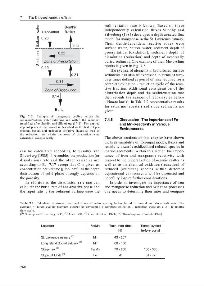
sedimentation rate is known. Based on these
independently calculated fluxes Sundby and
Silverberg (1985) developed a depth-zonated flux
model for manganese in the St. Lawrence estuary.
Their depth-dependent reactive zones were
surface water, bottom water, sediment depth of
precipitation (oxidation), sediment depth of
dissolution (reduction) and depth of eventually
buried sediment. One example of their Mn-cycling
results is given in Fig. 7.21.
The cycling of elements in bioturbated surface
sediments can also be expressed in terms of turnover times defined as period of time required for a
complete oxidation - reduction cycle of the reactive fraction. Additional consideration of the
bioturbation depth and the sedimentation rate
then reveals the number of redox-cycles before
ultimate burial. In Tab. 7.2 representative results
for estuarine (coastal) and slope sediments are
given.
7.4.5
Discussion: The Importance of Feand Mn-Reactivity in Various
Environments
The above sections of this chapter have shown
the high variability of iron-input modes, fluxes and
reactivity towards oxidized and reduced species in
marine sediments. Within this section the importance of iron and manganese reactivity with
respect to the mineralization of organic matter as
well as to the chemical oxidation (reduction) of
reduced (oxidized) species within different
depositional environments will be discussed and
hopefully inspire further considerations.
In order to investigate the importance of iron
and manganese reduction and oxidation processes
one needs to determine their rates and compare
Table 7.2 Calculated turn-over times and times of redox cycling before burial in coastal and slope sediments. The
dynamic of redox cycling becomes evident by envisaging a complete oxidation - reduction cycle on a 2 - 6 months
time scale.
( (1) Sundby and Silverberg 1985, (2) Aller 1980, (3) Canfield et al. 1993a, (4) Thamdrup and Canfield 1996)
Location
Fe/Mn
Turn-over time
Times cycled
[d]
before burial
St. Lawrence estuary
(1)
Mn
43 - 207
Long Island Sound estuary
(2)
Mn
60 - 100
Skagerrak
(3)
Fe/Mn
70 - 250
130 - 300
Slope off Chile
(4)
Fe
70
31 - 77
Zone of Precipitation
Zone of Dissolution
Burial
Deposition
Benthic
Reflux
Bottom water
Sediment
0.23
0.45
0.22
0.31
0.09
0.14
0.31
Fig. 7.21 Example of manganese cycling across the
sediment/bottom water interface and within the sediment
(modified after Sundby and Silverberg (1985). The applied
depth-dependent flux model is described in the text. Depositional, burial, and molecular diffusive fluxes as well as
the reduction rate within the zone of dissolution were
calculated independently.
The Biogeochemistry of Iron
260
can be calculated according to Sundby and
Silverberg (1985). P resembles the production (or
dissolution) rate and the other variables are
according to Eq. 7.17 except that C is given as
concentration per volume [µmol cm
-3
] as the depth
distribution of solid phase strongly depends on
the porosity.
In addition to the dissolution rate one can
calculate the burial rate of non-reactive phase and
the input rate to the sediment surface once the
sedimentation rate is known. Based on these
independently calculated fluxes Sundby and
Silverberg (1985) developed a depth-zonated flux
model for manganese in the St. Lawrence estuary.
Their depth-dependent reactive zones were
surface water, bottom water, sediment depth of
precipitation (oxidation), sediment depth of
dissolution (reduction) and depth of eventually
buried sediment. One example of their Mn-cycling
results is given in Fig. 7.21.
The cycling of elements in bioturbated surface
sediments can also be expressed in terms of turnover times defined as period of time required for a
complete oxidation - reduction cycle of the reactive fraction. Additional consideration of the
bioturbation depth and the sedimentation rate
then reveals the number of redox-cycles before
ultimate burial. In Tab. 7.2 representative results
for estuarine (coastal) and slope sediments are
given.
7.4.5
Discussion: The Importance of Feand Mn-Reactivity in Various
Environments
The above sections of this chapter have shown
the high variability of iron-input modes, fluxes and
reactivity towards oxidized and reduced species in
marine sediments. Within this section the importance of iron and manganese reactivity with
respect to the mineralization of organic matter as
well as to the chemical oxidation (reduction) of
reduced (oxidized) species within different
depositional environments will be discussed and
hopefully inspire further considerations.
In order to investigate the importance of iron
and manganese reduction and oxidation processes
one needs to determine their rates and compare
Table 7.2 Calculated turn-over times and times of redox cycling before burial in coastal and slope sediments. The
dynamic of redox cycling becomes evident by envisaging a complete oxidation - reduction cycle on a 2 - 6 months
time scale.
( (1) Sundby and Silverberg 1985, (2) Aller 1980, (3) Canfield et al. 1993a, (4) Thamdrup and Canfield 1996)
Location
Fe/Mn
Turn-over time
Times cycled
[d]
before burial
St. Lawrence estuary
(1)
Mn
43 - 207
Long Island Sound estuary
(2)
Mn
60 - 100
Skagerrak
(3)
Fe/Mn
70 - 250
130 - 300
Slope off Chile
(4)
Fe
70
31 - 77
Zone of Precipitation
Zone of Dissolution
Burial
Deposition
Benthic
Reflux
Bottom water
Sediment
0.23
0.45
0.22
0.31
0.09
0.14
0.31
Fig. 7.21 Example of manganese cycling across the
sediment/bottom water interface and within the sediment
(modified after Sundby and Silverberg (1985). The applied
depth-dependent flux model is described in the text. Depositional, burial, and molecular diffusive fluxes as well as
the reduction rate within the zone of dissolution were
calculated independently.