

• Steady State Dry Deposition Method (Smith et al. 1993; Petelski and Piskozub
2006);
• Statistical Wet Deposition Method (Lewis and Schwartz 2004);
• Whitecap Method (Monahan et al. 1986);
• Micrometeorological Methods: eddy correlation (Nilsson and Rannik 2001),
gradiental method (Petelski 2003; Petelski and Piskozub 2006; Andreas 2007)
• Multiple Methods (Lewis and Schwartz 2004);
The main disadvantage of all methods, except micrometeorological is the fact that
they are based on more qualitative estimation than direct flux determination. However, micrometeorological method and especially eddy correlation (EC) are more and
more popular in field measurements over open oceans. Micrometeorological Methods rely on strong physical foundations as Monin-Obukhov theory or Reynolds
Decomposition. Eddy covariance method (Lee et al. 2004; Aubinet et al. 2012) is
commonly used in air-sea gas transfer measurements, by using high frequency
concentration and wind speed measurements (*20 Hz, commonly used ultrasonic
anemometers work even with 50 Hz speed). Unfortunately, it is still impossible to
measure aerosol concentration with a frequency as high as in the case of trace gases.
However, thanks to technological progress, it is possible to construct increasingly
faster particle counters (*1 Hz is acceptable level, De Leeuw et al. 2007). During
SEASAW campaign (described by Norris et al. 2012) there was used A Compact
Lightweight Aerosol Spectrometer Probe (CLASP) which allows to measure aerosol
concentration with even 10 Hz speed in 0.24 μm < D p < 18.5 μm range. High
frequency measurements are necessary to record air turbulence spectrum. In fluid
dynamics there is common mathematical technique, which allow to separate average
x and fluctuating x′ parts of given quantity (Müller 2006; Foken and Nappo 2008):
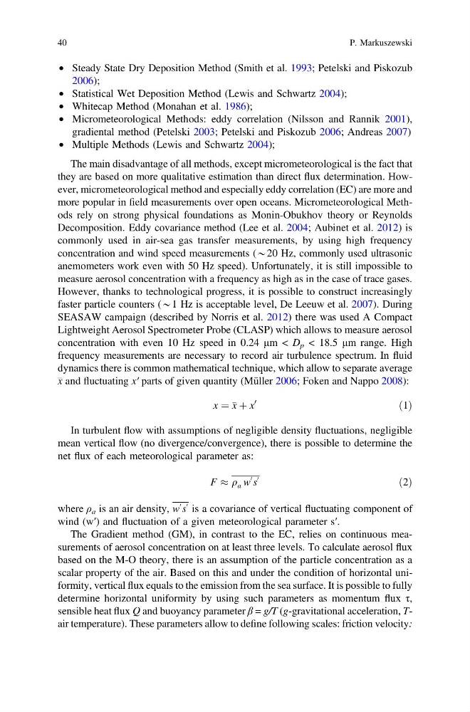
x ¼ x þ x
0
ð1Þ
In turbulent flow with assumptions of negligible density fluctuations, negligible
mean vertical flow (no divergence/convergence), there is possible to determine the
net flux of each meteorological parameter as:
F % q a w
0 s
0
ð2Þ
where ρ a is an air density, w
0 s
0 is a covariance of vertical fluctuating component of
wind (w′) and fluctuation of a given meteorological parameter s′.
The Gradient method (GM), in contrast to the EC, relies on continuous measurements of aerosol concentration on at least three levels. To calculate aerosol flux
based on the M-O theory, there is an assumption of the particle concentration as a
scalar property of the air. Based on this and under the condition of horizontal uniformity, vertical flux equals to the emission from the sea surface. It is possible to fully
determine horizontal uniformity by using such parameters as momentum flux τ,
sensible heat flux Q and buoyancy parameter β = g/T (g-gravitational acceleration, Tair temperature). These parameters allow to define following scales: friction velocity:
40
P. Markuszewski
2006);
• Statistical Wet Deposition Method (Lewis and Schwartz 2004);
• Whitecap Method (Monahan et al. 1986);
• Micrometeorological Methods: eddy correlation (Nilsson and Rannik 2001),
gradiental method (Petelski 2003; Petelski and Piskozub 2006; Andreas 2007)
• Multiple Methods (Lewis and Schwartz 2004);
The main disadvantage of all methods, except micrometeorological is the fact that
they are based on more qualitative estimation than direct flux determination. However, micrometeorological method and especially eddy correlation (EC) are more and
more popular in field measurements over open oceans. Micrometeorological Methods rely on strong physical foundations as Monin-Obukhov theory or Reynolds
Decomposition. Eddy covariance method (Lee et al. 2004; Aubinet et al. 2012) is
commonly used in air-sea gas transfer measurements, by using high frequency
concentration and wind speed measurements (*20 Hz, commonly used ultrasonic
anemometers work even with 50 Hz speed). Unfortunately, it is still impossible to
measure aerosol concentration with a frequency as high as in the case of trace gases.
However, thanks to technological progress, it is possible to construct increasingly
faster particle counters (*1 Hz is acceptable level, De Leeuw et al. 2007). During
SEASAW campaign (described by Norris et al. 2012) there was used A Compact
Lightweight Aerosol Spectrometer Probe (CLASP) which allows to measure aerosol
concentration with even 10 Hz speed in 0.24 μm < D p < 18.5 μm range. High
frequency measurements are necessary to record air turbulence spectrum. In fluid
dynamics there is common mathematical technique, which allow to separate average
x and fluctuating x′ parts of given quantity (Müller 2006; Foken and Nappo 2008):
x ¼ x þ x
0
ð1Þ
In turbulent flow with assumptions of negligible density fluctuations, negligible
mean vertical flow (no divergence/convergence), there is possible to determine the
net flux of each meteorological parameter as:
F % q a w
0 s
0
ð2Þ
where ρ a is an air density, w
0 s
0 is a covariance of vertical fluctuating component of
wind (w′) and fluctuation of a given meteorological parameter s′.
The Gradient method (GM), in contrast to the EC, relies on continuous measurements of aerosol concentration on at least three levels. To calculate aerosol flux
based on the M-O theory, there is an assumption of the particle concentration as a
scalar property of the air. Based on this and under the condition of horizontal uniformity, vertical flux equals to the emission from the sea surface. It is possible to fully
determine horizontal uniformity by using such parameters as momentum flux τ,
sensible heat flux Q and buoyancy parameter β = g/T (g-gravitational acceleration, Tair temperature). These parameters allow to define following scales: friction velocity:
40
P. Markuszewski