

284
Chapter 15: Multivariate Statistical Modeling:
identifying the second moment information by considering an AR(I) process
or by considering one cross-spectrum matrix is discussed in Section 15.3.4.
The latter is normally called a complex EOF analysis. In terms of one example, Section 15.4 considers the quest ion of to what extent the POPs can
be interpreted as normal mo des of the considered system.
15.2 The Cross-Covariance Matrix
and the Cross-Spectrum Matrix
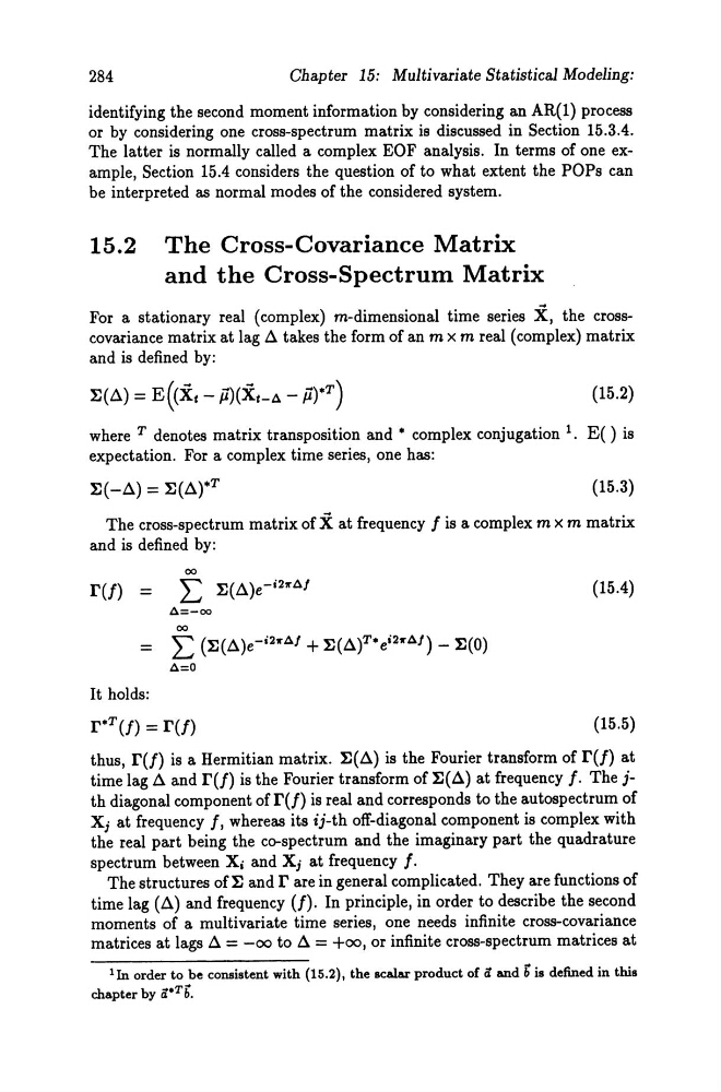
For a stationary real (complex) m-dimensional time series X, the crosscovariance matrix at lag Ll takes the form of an m x m real (complex) matrix
and is defined by:
(15.2)
where T denotes matrix transposition and • complex conjugation 1. E() is
expectation. For a complex time series, one has:
(15.3)
The cross-spectrum matrix of X at frequency / is a complex m x m matrix
and is defined by:
00
r(f) = l: E(Ll)e- i2 l1"AJ
(15.4)
A=-oo
00
= l: (E(Ll)e- i2 l1"AJ + E(Ll)T· ei21rAJ) - E(O)
A=O
It holds:
(15.5)
thus, r(f) is a Hermitian matrix. E(Ll) is the Fourier transform of r(f) at
time lag Ll and r(f) is the Fourier transform of E(Ll) at frequency /. The jth diagonal component of r(f) is real and corresponds to the autospectrum of
X j at frequency /, whereas its ij-th off-diagonal component is complex with
the real part being the co-spectrum and the imaginary part the quadrature
spectrum between Xi and Xj at frequency f.
The structures of E and r are in general complicated. They are functions of
time lag (Ll) and frequency (f). In principle, in order to describe the second
moments of a multivariate time series, one needs infinite cross-covariance
matrices at lags Ll = -00 to Ll = +00, or infinite cross-spectrum matrices at
11n order to be consistent with (15.2). the 8Calar product of ä and bis defined in this
chapter by äoTb.
Chapter 15: Multivariate Statistical Modeling:
identifying the second moment information by considering an AR(I) process
or by considering one cross-spectrum matrix is discussed in Section 15.3.4.
The latter is normally called a complex EOF analysis. In terms of one example, Section 15.4 considers the quest ion of to what extent the POPs can
be interpreted as normal mo des of the considered system.
15.2 The Cross-Covariance Matrix
and the Cross-Spectrum Matrix
For a stationary real (complex) m-dimensional time series X, the crosscovariance matrix at lag Ll takes the form of an m x m real (complex) matrix
and is defined by:
(15.2)
where T denotes matrix transposition and • complex conjugation 1. E() is
expectation. For a complex time series, one has:
(15.3)
The cross-spectrum matrix of X at frequency / is a complex m x m matrix
and is defined by:
00
r(f) = l: E(Ll)e- i2 l1"AJ
(15.4)
A=-oo
00
= l: (E(Ll)e- i2 l1"AJ + E(Ll)T· ei21rAJ) - E(O)
A=O
It holds:
(15.5)
thus, r(f) is a Hermitian matrix. E(Ll) is the Fourier transform of r(f) at
time lag Ll and r(f) is the Fourier transform of E(Ll) at frequency /. The jth diagonal component of r(f) is real and corresponds to the autospectrum of
X j at frequency /, whereas its ij-th off-diagonal component is complex with
the real part being the co-spectrum and the imaginary part the quadrature
spectrum between Xi and Xj at frequency f.
The structures of E and r are in general complicated. They are functions of
time lag (Ll) and frequency (f). In principle, in order to describe the second
moments of a multivariate time series, one needs infinite cross-covariance
matrices at lags Ll = -00 to Ll = +00, or infinite cross-spectrum matrices at
11n order to be consistent with (15.2). the 8Calar product of ä and bis defined in this
chapter by äoTb.