

Section 13.3: Empirical Orthogonal Functions
239
We have introduced EOFs as patterns which minimize the variance of the
residual (13.21). The variance depends on the chosen geometry, and we could
replace in (13.21) the square by a scalar product (-, -) such that
( ~
K
~k ~
K
~k )
€K = E (X - Ek=l ClkP ,X - Ek=l ClkP )
The EOF coeflicients are then also given as dot products
Clk(t) = (Xt,pk)
(13.25)
Obviously the result ofthe analysis depends on the choice ofthe dot product,
which is to some extend arbitrary.
13.3.2 What EOFs Are Not Designed for ...
There are some words of caution required when dealing with EOFs. These
patterns are constructed to represent in an optimal manner variance and covariance (in the sense ofjoint variance), not physical connections or maximum
correlation (see ehen and Harr, 1993). Therefore they are excellent tools to
compress data into a few variance-wise significant components. Sometimes
people expect more from EOFs, for instance a description of the "coherent
structures" (as, for instance, teleconnections). This goal can be achieved
only when the data are normalized to variance one, i.e., if the correlation
matrix instead of the covariance matrix is considered (see Wall ace and GutzIer, 1981). Another expectation is that EOFs would tell us something ab out
the structure of an underlying continuous field from which the data vector X
is sampled. Also often EOFs are thought to represent modes of "natural" or
"forced" variability. We will discuss these expectations in the following .
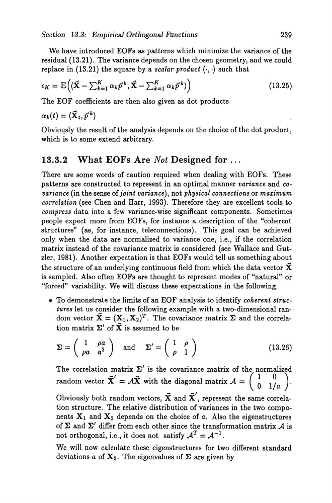
• To demonstrate the limits of an EOF analysis to identify coherent structures let us consider the following example with a two-dimensional random vector X = (Xl, x 2 )T. The covariance matrix ~ and the correlation matrix ~' of Xis assumed to be
(13.26)
The correlation matrix ~' is the covariance matrix of the normalized
random vector X' = AX with the diagonal matrix A = (~ 1~a)'
~
~,
Obviously both random vectors, X and X , represent the same correlation structure. The relative distribution of variances in the two components Xl and X2 depends on the choice of a. Also the eigenstructures
of ~ and ~' differ from each other since the transformation matrix A is
not orthogonal, i.e., it does not satisfy AT = A- l .
We will now calculate these eigenstructures for two different standard
deviations a of X 2 • The eigenvalues of ~ are given by
239
We have introduced EOFs as patterns which minimize the variance of the
residual (13.21). The variance depends on the chosen geometry, and we could
replace in (13.21) the square by a scalar product (-, -) such that
( ~
K
~k ~
K
~k )
€K = E (X - Ek=l ClkP ,X - Ek=l ClkP )
The EOF coeflicients are then also given as dot products
Clk(t) = (Xt,pk)
(13.25)
Obviously the result ofthe analysis depends on the choice ofthe dot product,
which is to some extend arbitrary.
13.3.2 What EOFs Are Not Designed for ...
There are some words of caution required when dealing with EOFs. These
patterns are constructed to represent in an optimal manner variance and covariance (in the sense ofjoint variance), not physical connections or maximum
correlation (see ehen and Harr, 1993). Therefore they are excellent tools to
compress data into a few variance-wise significant components. Sometimes
people expect more from EOFs, for instance a description of the "coherent
structures" (as, for instance, teleconnections). This goal can be achieved
only when the data are normalized to variance one, i.e., if the correlation
matrix instead of the covariance matrix is considered (see Wall ace and GutzIer, 1981). Another expectation is that EOFs would tell us something ab out
the structure of an underlying continuous field from which the data vector X
is sampled. Also often EOFs are thought to represent modes of "natural" or
"forced" variability. We will discuss these expectations in the following .
• To demonstrate the limits of an EOF analysis to identify coherent structures let us consider the following example with a two-dimensional random vector X = (Xl, x 2 )T. The covariance matrix ~ and the correlation matrix ~' of Xis assumed to be
(13.26)
The correlation matrix ~' is the covariance matrix of the normalized
random vector X' = AX with the diagonal matrix A = (~ 1~a)'
~
~,
Obviously both random vectors, X and X , represent the same correlation structure. The relative distribution of variances in the two components Xl and X2 depends on the choice of a. Also the eigenstructures
of ~ and ~' differ from each other since the transformation matrix A is
not orthogonal, i.e., it does not satisfy AT = A- l .
We will now calculate these eigenstructures for two different standard
deviations a of X 2 • The eigenvalues of ~ are given by