

240
Ghapter 13: Spatial Patterns: EOFs and GGA
A1,2 = ~ [1 + a 2 ± J1 - 2a 2 + a 4 + 4(pa)2]
(13.27)
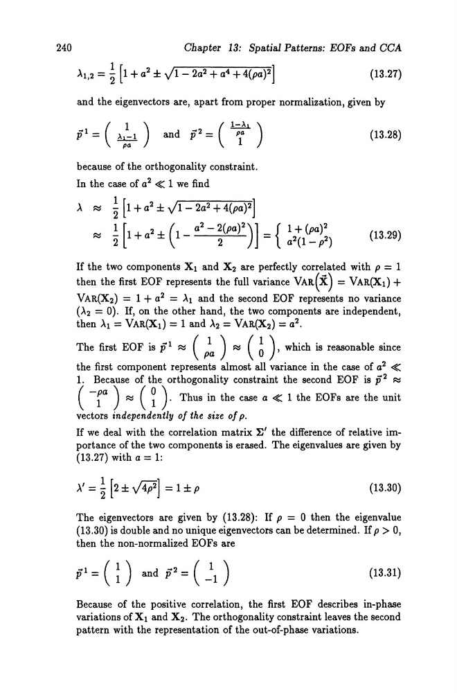
and the eigenvectors are, apart from proper normalization, given by
because of the orthogonality constraint.
In the case of a 2 ~ 1 we find
A ~ ~ [1 + a 2 ± J1- 2a 2 + 4(pa)2]
~ ~ [1 + a 2 ± (1 _ a 2 - ~(pa)2) ] = {
(13.28)
(13.29)
If the two components Xl and X2 are perfectly correlated with p = 1
then the first EOF represents the fun variance VAR(X) = VAR(Xt} +
VAR(X2) = 1 + a 2 = Al and the second EOF represents no variance
(>'2 = 0). If, on the other hand, the two components are independent,
then >' 1 = VAR(Xt} = 1 and >' 2 = VAR(X2) = a 2 •
The first EOF is p1 ~ ( P: ) ~ ( ~ ), which is reasonable since
the first component represents almost an variance in the case of a 2 ~
1. Because of the orthogonality constraint the second EOF is p2 ~
( -ra ) ~ ( ~ ). Thus in the case a ~ 1 the EOFs are the unit
vectors independently oi the size oi p.
If we deal with the correlation matrix ~' the difference of relative importance of the two components is erased. The eigenvalues are given by
(13.27) with a = 1:
>.' = ~ [2 ± N] = 1 ± p
(13.30)
The eigenvectors are given by (13.28): If p = 0 then the eigenvalue
(13.30) is double and no unique eigenvectors can be determined. If p > 0,
then the non-normalized EOFs are
(13.31 )
Because of the positive correlation, the first EOF describes in-phase
variations of Xl and X2• The orthogonality constraint leaves the second
pattern with the representation of the out-of-phase variations.
Ghapter 13: Spatial Patterns: EOFs and GGA
A1,2 = ~ [1 + a 2 ± J1 - 2a 2 + a 4 + 4(pa)2]
(13.27)
and the eigenvectors are, apart from proper normalization, given by
because of the orthogonality constraint.
In the case of a 2 ~ 1 we find
A ~ ~ [1 + a 2 ± J1- 2a 2 + 4(pa)2]
~ ~ [1 + a 2 ± (1 _ a 2 - ~(pa)2) ] = {
(13.28)
(13.29)
If the two components Xl and X2 are perfectly correlated with p = 1
then the first EOF represents the fun variance VAR(X) = VAR(Xt} +
VAR(X2) = 1 + a 2 = Al and the second EOF represents no variance
(>'2 = 0). If, on the other hand, the two components are independent,
then >' 1 = VAR(Xt} = 1 and >' 2 = VAR(X2) = a 2 •
The first EOF is p1 ~ ( P: ) ~ ( ~ ), which is reasonable since
the first component represents almost an variance in the case of a 2 ~
1. Because of the orthogonality constraint the second EOF is p2 ~
( -ra ) ~ ( ~ ). Thus in the case a ~ 1 the EOFs are the unit
vectors independently oi the size oi p.
If we deal with the correlation matrix ~' the difference of relative importance of the two components is erased. The eigenvalues are given by
(13.27) with a = 1:
>.' = ~ [2 ± N] = 1 ± p
(13.30)
The eigenvectors are given by (13.28): If p = 0 then the eigenvalue
(13.30) is double and no unique eigenvectors can be determined. If p > 0,
then the non-normalized EOFs are
(13.31 )
Because of the positive correlation, the first EOF describes in-phase
variations of Xl and X2• The orthogonality constraint leaves the second
pattern with the representation of the out-of-phase variations.