

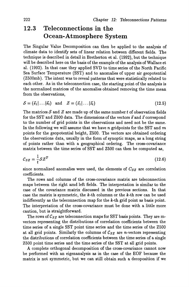
222
Chapter 12: Teleconnections Patterns
12.3 Teleconnections in the
Ocean-Atmosphere System
The Singular Value Decomposition can then be applied to the analysis of
climate data to identify sets of linear relation between different fields. The
technique is described in detail in Bretherton et al. (1992), but the technique
will be described here on the basis of the example of the analysis of Wall ace et
al. (1992). In that case they applied SVD to time series of the North Pacific
Sea Surface Temperature (SST) and to anomalies of upper air geopotential
(Z500mb). The intent was to reveal patterns that were statistically related to
each other. As in the teleconnection case, the starting point of the analysis is
the normalized matrices of the anomalies obtained removing the time mean
from the observations,
(12.5)
The matrices Sand Z are made up of the same number t of observation fields
for the SST and Z500 data. The dimensions of the vectors ; and z correspond
to the number of grid points in the observations and need not be the same.
In the following we will assurne that we have n gridpoints for the SST and m
points for the geopotential height, Z500. The vectors are obtained ordering
the observations data, usually in the form of synoptic maps, as a long string
of points rather than with a geographical ordering. The cross-covariance
matrix between the time series of SST and Z500 can then be computed as,
1 T
Csz = 'i SZ
(12.6)
sinee normalized anomalies were used, the elements of Csz are eorrelation
coeffieients.
The rows and eolumns of the eross-covariance matrix are teleeonnection
maps between the right amd left fields. The interpretation is similar to the
ease of the covarianee matrix diseussed in the previous sections. In that
ease the matrix is symmetrie, the k-th eolumnn or the k-th row ean be used
indifferently as the teleeonnection map for the k-th grid point as basis point.
The interpretation of the eross-eovarianee must be done with a little more
eaution, but is straightforward.
The rows of Csz are teleeonnection maps for SST basis points. They are mvectors representing the distributions of eorrelation eoefficients between the
time series of a single SST point time series and the time series of the Z500
at all grid points. Similarly the eolumns of Csz are n-vectors representing
the distributions of correlation coefficients between the time series of a single
Z500 point time series and the time series of the SST at all grid points.
A eomplete orthogonal deeomposition of the eross-eovarianee cannot now
be performed with an eigenanalysis as in the ease of the EOF beeause the
matrix is not symmetrie, but we ean still obtain such a deeoposition if we
Chapter 12: Teleconnections Patterns
12.3 Teleconnections in the
Ocean-Atmosphere System
The Singular Value Decomposition can then be applied to the analysis of
climate data to identify sets of linear relation between different fields. The
technique is described in detail in Bretherton et al. (1992), but the technique
will be described here on the basis of the example of the analysis of Wall ace et
al. (1992). In that case they applied SVD to time series of the North Pacific
Sea Surface Temperature (SST) and to anomalies of upper air geopotential
(Z500mb). The intent was to reveal patterns that were statistically related to
each other. As in the teleconnection case, the starting point of the analysis is
the normalized matrices of the anomalies obtained removing the time mean
from the observations,
(12.5)
The matrices Sand Z are made up of the same number t of observation fields
for the SST and Z500 data. The dimensions of the vectors ; and z correspond
to the number of grid points in the observations and need not be the same.
In the following we will assurne that we have n gridpoints for the SST and m
points for the geopotential height, Z500. The vectors are obtained ordering
the observations data, usually in the form of synoptic maps, as a long string
of points rather than with a geographical ordering. The cross-covariance
matrix between the time series of SST and Z500 can then be computed as,
1 T
Csz = 'i SZ
(12.6)
sinee normalized anomalies were used, the elements of Csz are eorrelation
coeffieients.
The rows and eolumns of the eross-covariance matrix are teleeonnection
maps between the right amd left fields. The interpretation is similar to the
ease of the covarianee matrix diseussed in the previous sections. In that
ease the matrix is symmetrie, the k-th eolumnn or the k-th row ean be used
indifferently as the teleeonnection map for the k-th grid point as basis point.
The interpretation of the eross-eovarianee must be done with a little more
eaution, but is straightforward.
The rows of Csz are teleeonnection maps for SST basis points. They are mvectors representing the distributions of eorrelation eoefficients between the
time series of a single SST point time series and the time series of the Z500
at all grid points. Similarly the eolumns of Csz are n-vectors representing
the distributions of correlation coefficients between the time series of a single
Z500 point time series and the time series of the SST at all grid points.
A eomplete orthogonal deeomposition of the eross-eovarianee cannot now
be performed with an eigenanalysis as in the ease of the EOF beeause the
matrix is not symmetrie, but we ean still obtain such a deeoposition if we