

86
P. Courtier
a background is not necessarily included is presented (in a very accessible way) in Tarantola
(1987). The analysis value is obtained for a given realization of the background and the observations replacing the random variables in (4.4) by their values.
In meteorology the practical difficulty is that it is impossible to use (4.4) and (4.5) directly.
B, for example, is a matrix of size 10 7 x 10 7 which is about 1000 times the total archiving
capabilities of ECMWF and one million times the memory size of the current computers.
The scientific difficulty of data assimilation is then to find algorithms which simplify (4.4) and
(4.5) to an affordable amount of computer resources, while preserving some of the essential
characters.
4.2.3 Quasi linear case
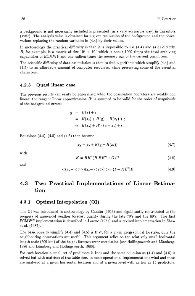
The previous results can easily be generalised when the observation operators are weakly non
linear: the tangent linear approximation H' is assumed to be valid for the order of magnitude
of the background errors:
J!..
H(:£) + f
H(Xb) + H(:£) - H(Xb) + f
' :::' H(Xb) + H' . (:£ - Xb) + f.
Equations (4.4), (4.5) and (4.6) then become
with
and
< (;r.a -= (1- KH')B.
( 4.7)
( 4.8)
( 4.9)
4.3 Two Practical Implementations of Linear Estimation
4.3.1 Optimal Interpolation (01)
The 01 was introduced in meteorology by Gandin (1963) and significantly contributed to the
progress of numerical weather forecast quality during the late 70's and the 80's. The first
ECMWF implementation is described in Lorenc (1981) and a revised implementation in Shaw
et al. (1987).
The basic idea to simplify (4.4) and (4.5) is that, for a given geographical location, only the
neighbouring observations are useful. This argument relies on the relatively small horizontal
length scale (500 km) of the height forecast error correlation (see Hollingsworth and Lonnberg,
1986 and Lonnberg and Hollingsworth, 1986).
For each location a small set of predictors is kept and the same equation as (4.4) and (4.5) is
solved but with matrices of tractable size. In some operational implementations wind and mass
are analysed at a given horizontal location and at a given level with as few as 15 predictors.
P. Courtier
a background is not necessarily included is presented (in a very accessible way) in Tarantola
(1987). The analysis value is obtained for a given realization of the background and the observations replacing the random variables in (4.4) by their values.
In meteorology the practical difficulty is that it is impossible to use (4.4) and (4.5) directly.
B, for example, is a matrix of size 10 7 x 10 7 which is about 1000 times the total archiving
capabilities of ECMWF and one million times the memory size of the current computers.
The scientific difficulty of data assimilation is then to find algorithms which simplify (4.4) and
(4.5) to an affordable amount of computer resources, while preserving some of the essential
characters.
4.2.3 Quasi linear case
The previous results can easily be generalised when the observation operators are weakly non
linear: the tangent linear approximation H' is assumed to be valid for the order of magnitude
of the background errors:
J!..
H(:£) + f
H(Xb) + H(:£) - H(Xb) + f
' :::' H(Xb) + H' . (:£ - Xb) + f.
Equations (4.4), (4.5) and (4.6) then become
with
and
< (;r.a -
( 4.7)
( 4.8)
( 4.9)
4.3 Two Practical Implementations of Linear Estimation
4.3.1 Optimal Interpolation (01)
The 01 was introduced in meteorology by Gandin (1963) and significantly contributed to the
progress of numerical weather forecast quality during the late 70's and the 80's. The first
ECMWF implementation is described in Lorenc (1981) and a revised implementation in Shaw
et al. (1987).
The basic idea to simplify (4.4) and (4.5) is that, for a given geographical location, only the
neighbouring observations are useful. This argument relies on the relatively small horizontal
length scale (500 km) of the height forecast error correlation (see Hollingsworth and Lonnberg,
1986 and Lonnberg and Hollingsworth, 1986).
For each location a small set of predictors is kept and the same equation as (4.4) and (4.5) is
solved but with matrices of tractable size. In some operational implementations wind and mass
are analysed at a given horizontal location and at a given level with as few as 15 predictors.