

Introduction to Numerical Weather Prediction Data Assimilation
87
At ECMWF, a box of a typical size 500 km is considered and an order of magnitude of 700
predictors is kept.
The second approximation comes from the necessity of an analytical model for the forecast
error covariances which have to be computed at the observation locations. This model in most
(all?) implementations relies on isotropy and geostrophy on the f-plane (f is assumed instant
locally) with a separability vertical/horizontal (the spatial correlations can be expressed as a
product of two functions, one which depends on the horizontal distance only and one on the
vertical distance only).
Generally speaking, the more local, the more noisy the analyses are (there are jumps in the
data used from one location to another). A second weakness of 01 is that if, in principle, any
linear (or linearised) observation operator may be used, it is difficult to practically make use
of observations indirectly related to the model parameters since in (4.5) all the forecast error
covariances in observation space have to be computed. Durand (1985) implemented a direct
use of satellite radiances but it significantly increased the PERIDOT 01 code complexity.
The analysis error variances are easily computed using (4.6) for each simplified problem.
4.3.2 Variational formulation of linear estimation - 3D-Var
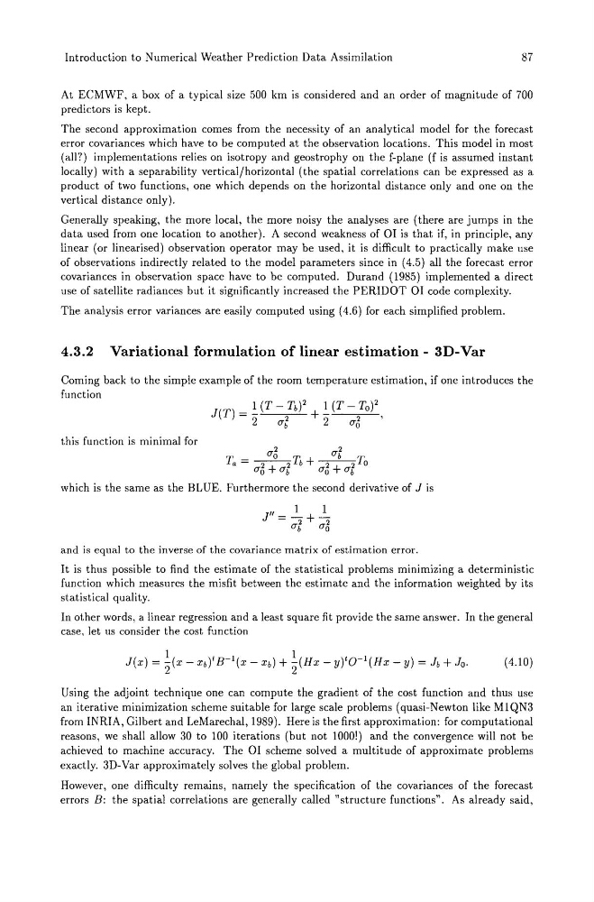
Coming back to the simple example of the room temperature estimation, if one introduces the
function
this function is minimal for
U 2
u 2
Ta=~n+~To
U o + Ub
U o + Ub
which is the same as the BLUE. Furthermore the second derivative of J is
and is equal to the inverse of the covariance matrix of estimation error.
It is thus possible to find the estimate of the statistical problems minimizing a deterministic
function which measures the misfit between the estimate and the information weighted by its
statistical quality.
In other words, a linear regression and a least square fit provide the same answer. In the general
case, let us consider the cost function
(4.10)
Using the adjoint technique one can compute the gradient of the cost function and thus use
an iterative minimization scheme suitable for large scale problems (quasi-Newton like M1QN3
from INRIA, Gilbert and LeMarechal, 1989). Here is the first approximation: for computational
reasons, we shall allow 30 to 100 iterations (but not 1000!) and the convergence will not be
achieved to machine accuracy. The 01 scheme solved a multitude of approximate problems
exactly. 30-Var approximately solves the global problem.
However, one difficulty remains, namely the specification of the covariances of the forecast
errors B: the spatial correlations are generally called "structure functions". As already said,
87
At ECMWF, a box of a typical size 500 km is considered and an order of magnitude of 700
predictors is kept.
The second approximation comes from the necessity of an analytical model for the forecast
error covariances which have to be computed at the observation locations. This model in most
(all?) implementations relies on isotropy and geostrophy on the f-plane (f is assumed instant
locally) with a separability vertical/horizontal (the spatial correlations can be expressed as a
product of two functions, one which depends on the horizontal distance only and one on the
vertical distance only).
Generally speaking, the more local, the more noisy the analyses are (there are jumps in the
data used from one location to another). A second weakness of 01 is that if, in principle, any
linear (or linearised) observation operator may be used, it is difficult to practically make use
of observations indirectly related to the model parameters since in (4.5) all the forecast error
covariances in observation space have to be computed. Durand (1985) implemented a direct
use of satellite radiances but it significantly increased the PERIDOT 01 code complexity.
The analysis error variances are easily computed using (4.6) for each simplified problem.
4.3.2 Variational formulation of linear estimation - 3D-Var
Coming back to the simple example of the room temperature estimation, if one introduces the
function
this function is minimal for
U 2
u 2
Ta=~n+~To
U o + Ub
U o + Ub
which is the same as the BLUE. Furthermore the second derivative of J is
and is equal to the inverse of the covariance matrix of estimation error.
It is thus possible to find the estimate of the statistical problems minimizing a deterministic
function which measures the misfit between the estimate and the information weighted by its
statistical quality.
In other words, a linear regression and a least square fit provide the same answer. In the general
case, let us consider the cost function
(4.10)
Using the adjoint technique one can compute the gradient of the cost function and thus use
an iterative minimization scheme suitable for large scale problems (quasi-Newton like M1QN3
from INRIA, Gilbert and LeMarechal, 1989). Here is the first approximation: for computational
reasons, we shall allow 30 to 100 iterations (but not 1000!) and the convergence will not be
achieved to machine accuracy. The 01 scheme solved a multitude of approximate problems
exactly. 30-Var approximately solves the global problem.
However, one difficulty remains, namely the specification of the covariances of the forecast
errors B: the spatial correlations are generally called "structure functions". As already said,