Model Development for Passive Microwave Remote Sensing ...
579
21.3.1.1 Emission simulation
In this section the emission simulation as part of the MIMR-software is briefly described (Pulliainen et al., 1990). Emittance models are implemented to simulate the surface emittance Es
from
- ocean surface using Pandey's or Wilheit's model (Pandey et al., 1982, Wilheit, 1979),
- snow-covered land using HUT's model (Hallikainen et al., 1988),
- vegetation covered land using Kerr's model (Pulliainen et al., 1990), and
- different ice types using constant emittance values.
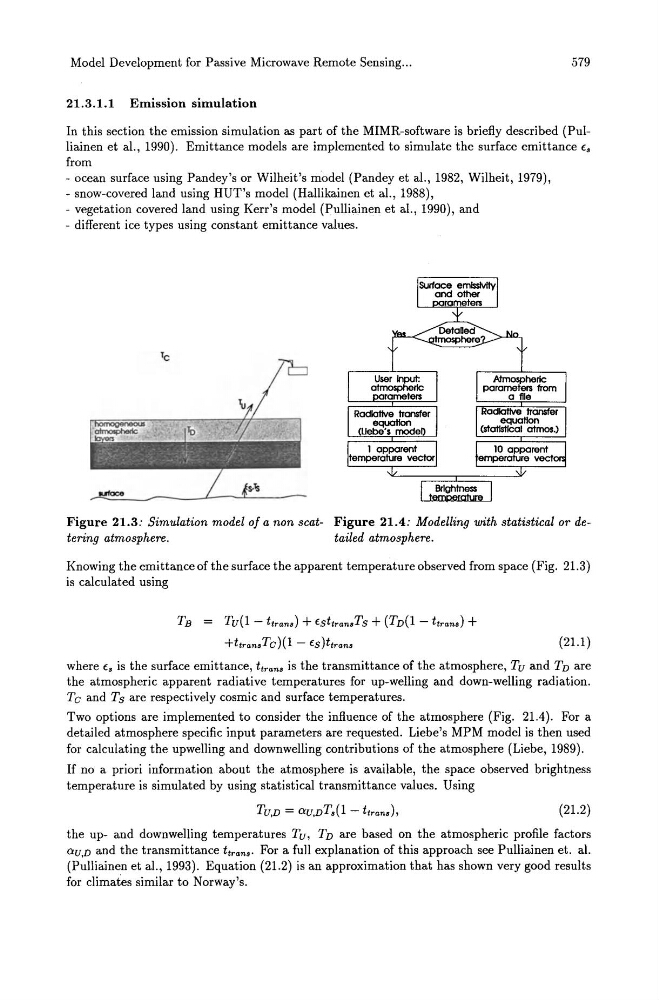
Figure 21.3: Simulation model of a non scat- Figure 21.4: Modelling with statistical or detering atmosphere.
tailed atmosphere.
Knowing the emittance of the surface the apparent temperature observed from space (Fig. 21.3)
is calculated using
TB
Tu(1 - ttrans) + EsttransTs + (TD(1 - ttrans) +
+ttransTc )(1 - ES )ttrans
(21.1 )
where Es is the surface emittance, ttrans is the transmittance of the atmosphere, Tu and TD are
the atmospheric apparent radiative temperatures for up-welling and down-welling radiation.
Tc and Ts are respectively cosmic and surface temperatures.
Two options are implemented to consider the influence of the atmosphere (Fig. 21.4). For a
detailed atmosphere specific input parameters are requested. Liebe's MPM model is then used
for calculating the upwelling and downwelling contributions of the atmosphere (Liebe, 1989).
If no a priori information about the atmosphere is available, the space observed brightness
temperature is simulated by using statistical transmittance values. Using
TU,D = au,DT.(1 - ttrans),
(21.2)
the up- and downwelling temperatures Tu, TD are based on the atmospheric profile factors
aU,D and the transmittance ttrans. For a full explanation of this approach see Pulliainen et. al.
(Pulliainen et al., 1993). Equation (21.2) is an approximation that has shown very good results
for climates similar to Norway's.