

472
K.B. Katsaros
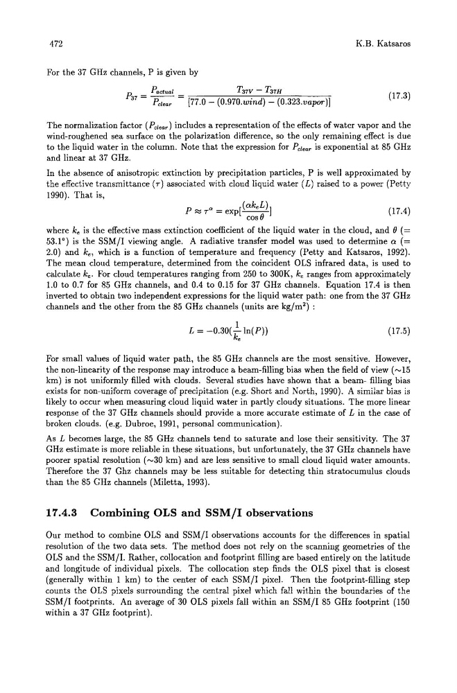
For the 37 GHz channels, P is given by
P 37 = Pactual =
T 37V - T37H
Pc/ear
[77.0 - (0.970.wind) - (0.323.vapor)]
(17.3)
The normalization factor (Pc/ear) includes a representation of the effects of water vapor and the
wind-roughened sea surface on the polarization difference, so the only remaining effect is due
to the liquid water in the column. Note that the expression for Pc/ear is exponential at 85 GHz
and linear at 37 GHz.
In the absence of anisotropic extinction by precipitation particles, P is well approximated by
the effective transmittance (T) associated with cloud liquid water (L) raised to a power (Petty
1990). That is,
P
a
[(ake L )]
~T =exp cosO
(17.4)
where ke is the effective mass extinction coefficient of the liquid water in the cloud, and 0 (=
53.1 0 ) is the SSM/I viewing angle. A radiative transfer model was used to determine a (=
2.0) and ke, which is a function of temperature and frequency (Petty and Katsaros, 1992).
The mean cloud temperature, determined from the coincident OLS infrared data, is used to
calculate ke • For cloud temperatures ranging from 250 to 300K, ke ranges from approximately
1.0 to 0.7 for 85 GHz channels, and 0.4 to 0.15 for 37 GHz channels. Equation 17.4 is then
inverted to obtain two independent expressions for the liquid water path: one from the 37 GHz
channels and the other from the 85 GHz channels (units are kg/m 2 ) :
1
L = -0.30( ke In( P))
(17.5)
For small values of liquid water path, the 85 GHz channels are the most sensitive. However,
the non-linearity of the response may introduce a beam-filling bias when the field of view ('" 15
km) is not uniformly filled with clouds. Several studies have shown that a beam- filling bias
exists for non-uniform coverage of precipitation (e.g. Short and North, 1990). A similar bias is
likely to occur when measuring cloud liquid water in partly cloudy situations. The more linear
response of the 37 GHz channels should provide a more accurate estimate of L in the case of
broken clouds. (e.g. Dubroe, 1991, personal communication).
As L becomes large, the 85 GHz channels tend to saturate and lose their sensitivity. The 37
GHz estimate is more reliable in these situations, but unfortunately, the 37 GHz channels have
poorer spatial resolution (",30 km) and are less sensitive to small cloud liquid water amounts.
Therefore the 37 Ghz channels may be less suitable for detecting thin stratocumulus clouds
than the 85 GHz channels (Miletta, 1993).
17.4.3 Combining OLS and SSM/I observations
Our method to combine OLS and SSM/I observations accounts for the differences in spatial
resolution of the two data sets. The method does not rely on the scanning geometries of the
OLS and the SSM/I. Rather, collocation and footprint filling are based entirely on the latitude
and longitude of individual pixels. The collocation step finds the OLS pixel that is closest
(generally within 1 km) to the center of each SSM/I pixel. Then the footprint-filling step
counts the OLS pixels surrounding the central pixel which fall within the boundaries of the
SSM/I footprints. An average of 30 OLS pixels fall within an SSM/I 85 GHz footprint (150
within a 37 GHz footprint).
K.B. Katsaros
For the 37 GHz channels, P is given by
P 37 = Pactual =
T 37V - T37H
Pc/ear
[77.0 - (0.970.wind) - (0.323.vapor)]
(17.3)
The normalization factor (Pc/ear) includes a representation of the effects of water vapor and the
wind-roughened sea surface on the polarization difference, so the only remaining effect is due
to the liquid water in the column. Note that the expression for Pc/ear is exponential at 85 GHz
and linear at 37 GHz.
In the absence of anisotropic extinction by precipitation particles, P is well approximated by
the effective transmittance (T) associated with cloud liquid water (L) raised to a power (Petty
1990). That is,
P
a
[(ake L )]
~T =exp cosO
(17.4)
where ke is the effective mass extinction coefficient of the liquid water in the cloud, and 0 (=
53.1 0 ) is the SSM/I viewing angle. A radiative transfer model was used to determine a (=
2.0) and ke, which is a function of temperature and frequency (Petty and Katsaros, 1992).
The mean cloud temperature, determined from the coincident OLS infrared data, is used to
calculate ke • For cloud temperatures ranging from 250 to 300K, ke ranges from approximately
1.0 to 0.7 for 85 GHz channels, and 0.4 to 0.15 for 37 GHz channels. Equation 17.4 is then
inverted to obtain two independent expressions for the liquid water path: one from the 37 GHz
channels and the other from the 85 GHz channels (units are kg/m 2 ) :
1
L = -0.30( ke In( P))
(17.5)
For small values of liquid water path, the 85 GHz channels are the most sensitive. However,
the non-linearity of the response may introduce a beam-filling bias when the field of view ('" 15
km) is not uniformly filled with clouds. Several studies have shown that a beam- filling bias
exists for non-uniform coverage of precipitation (e.g. Short and North, 1990). A similar bias is
likely to occur when measuring cloud liquid water in partly cloudy situations. The more linear
response of the 37 GHz channels should provide a more accurate estimate of L in the case of
broken clouds. (e.g. Dubroe, 1991, personal communication).
As L becomes large, the 85 GHz channels tend to saturate and lose their sensitivity. The 37
GHz estimate is more reliable in these situations, but unfortunately, the 37 GHz channels have
poorer spatial resolution (",30 km) and are less sensitive to small cloud liquid water amounts.
Therefore the 37 Ghz channels may be less suitable for detecting thin stratocumulus clouds
than the 85 GHz channels (Miletta, 1993).
17.4.3 Combining OLS and SSM/I observations
Our method to combine OLS and SSM/I observations accounts for the differences in spatial
resolution of the two data sets. The method does not rely on the scanning geometries of the
OLS and the SSM/I. Rather, collocation and footprint filling are based entirely on the latitude
and longitude of individual pixels. The collocation step finds the OLS pixel that is closest
(generally within 1 km) to the center of each SSM/I pixel. Then the footprint-filling step
counts the OLS pixels surrounding the central pixel which fall within the boundaries of the
SSM/I footprints. An average of 30 OLS pixels fall within an SSM/I 85 GHz footprint (150
within a 37 GHz footprint).