

Remote Sensing Parameterization of Meso-scale ...
Sensible heat flux Wm- 2
400
300
200
_1
c::::J 2
c::::J 3
c::::J 4
c::::J 5
417
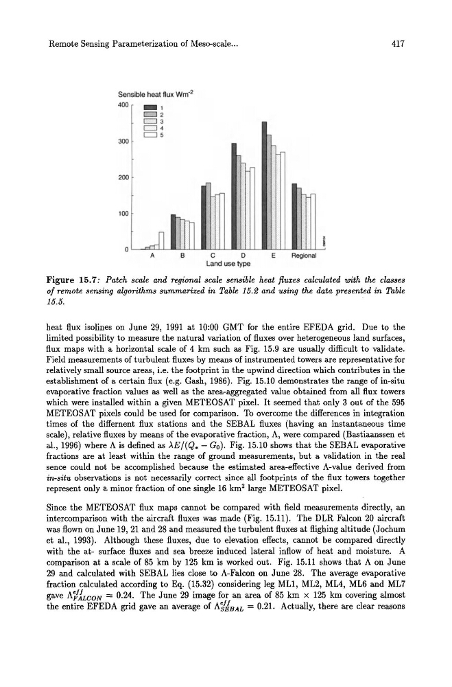
Figure 15.7: Patch scale and regional scale sensible heat fluxes calculated with the classes
of remote sensing algorithms summarized in Table 15.2 and using the data presented in Table
15.5.
heat flux isolines on June 29, 1991 at 10:00 GMT for the entire EFEDA grid. Due to the
limited possibility to measure the natural variation of fluxes over heterogeneous land surfaces,
flux maps with a horizontal scale of 4 km such as Fig. 15.9 are usually difficult to validate.
Field measurements of turbulent fluxes by means of instrumented towers are representative for
relatively small source areas, i.e. the footprint in the upwind direction which contributes in the
establishment of a certain flux (e.g. Gash, 1986). Fig. 15.10 demonstrates the range of in-situ
evaporative fraction values as well as the area-aggregated value obtained from all flux towers
which were installed within a given METEOSAT pixel. It seemed that only 3 out of the 595
METEOSAT pixels could be used for comparison. To overcome the differences in integration
times of the differnent flux stations and the SEBAL fluxes (having an instantaneous time
scale), relative fluxes by means of the evaporative fraction, A, were compared (Bastiaanssen et
al., 1996) where A is defined as )"E/(Q. - Go). Fig. 15.10 shows that the SEBAL evaporative
fractions are at least within the range of ground measurements, but a validation in the real
sence could not be accomplished because the estimated area-effective A-value derived from
in-situ observations is not necessarily correct since all footprints of the flux towers together
represent only a minor fraction of one single 16 km 2 large METEOSAT pixel.
Since the METEOSAT flux maps cannot be compared with field measurements directly, an
intercomparison with the aircraft fluxes was made (Fig. 15.11). The DLR Falcon 20 aircraft
was flown on June 19, 21 and 28 and measured the turbulent fluxes at flighing altitude (Jochum
et al., 1993). Although these fluxes, due to elevation effects, cannot be compared directly
with the at- surface fluxes and sea breeze induced lateral inflow of heat and moisture. A
comparison at a scale of 85 km by 125 km is worked out. Fig. 15.11 shows that A on June
29 and calculated with SEBAL lies close to A-Falcon on June 28. The average evaporative
fraction calculated according to Eq. (15.32) considering leg ML1, ML2, ML4, ML6 and ML7
gave A"/iwON = 0.24. The June 29 image for an area of 85 km x 125 km covering almost
the entire EFEDA grid gave an average of A"/JBAL = 0.21. Actually, there are clear reasons
Sensible heat flux Wm- 2
400
300
200
_1
c::::J 2
c::::J 3
c::::J 4
c::::J 5
417
Figure 15.7: Patch scale and regional scale sensible heat fluxes calculated with the classes
of remote sensing algorithms summarized in Table 15.2 and using the data presented in Table
15.5.
heat flux isolines on June 29, 1991 at 10:00 GMT for the entire EFEDA grid. Due to the
limited possibility to measure the natural variation of fluxes over heterogeneous land surfaces,
flux maps with a horizontal scale of 4 km such as Fig. 15.9 are usually difficult to validate.
Field measurements of turbulent fluxes by means of instrumented towers are representative for
relatively small source areas, i.e. the footprint in the upwind direction which contributes in the
establishment of a certain flux (e.g. Gash, 1986). Fig. 15.10 demonstrates the range of in-situ
evaporative fraction values as well as the area-aggregated value obtained from all flux towers
which were installed within a given METEOSAT pixel. It seemed that only 3 out of the 595
METEOSAT pixels could be used for comparison. To overcome the differences in integration
times of the differnent flux stations and the SEBAL fluxes (having an instantaneous time
scale), relative fluxes by means of the evaporative fraction, A, were compared (Bastiaanssen et
al., 1996) where A is defined as )"E/(Q. - Go). Fig. 15.10 shows that the SEBAL evaporative
fractions are at least within the range of ground measurements, but a validation in the real
sence could not be accomplished because the estimated area-effective A-value derived from
in-situ observations is not necessarily correct since all footprints of the flux towers together
represent only a minor fraction of one single 16 km 2 large METEOSAT pixel.
Since the METEOSAT flux maps cannot be compared with field measurements directly, an
intercomparison with the aircraft fluxes was made (Fig. 15.11). The DLR Falcon 20 aircraft
was flown on June 19, 21 and 28 and measured the turbulent fluxes at flighing altitude (Jochum
et al., 1993). Although these fluxes, due to elevation effects, cannot be compared directly
with the at- surface fluxes and sea breeze induced lateral inflow of heat and moisture. A
comparison at a scale of 85 km by 125 km is worked out. Fig. 15.11 shows that A on June
29 and calculated with SEBAL lies close to A-Falcon on June 28. The average evaporative
fraction calculated according to Eq. (15.32) considering leg ML1, ML2, ML4, ML6 and ML7
gave A"/iwON = 0.24. The June 29 image for an area of 85 km x 125 km covering almost
the entire EFEDA grid gave an average of A"/JBAL = 0.21. Actually, there are clear reasons