

410
W.G.M. Bastiaanssen
be assumed for each separated pixel and step-changes in surface conditions are schematized
at the pixel edges (if the image comprises a composite land surface). If the size of a pixel
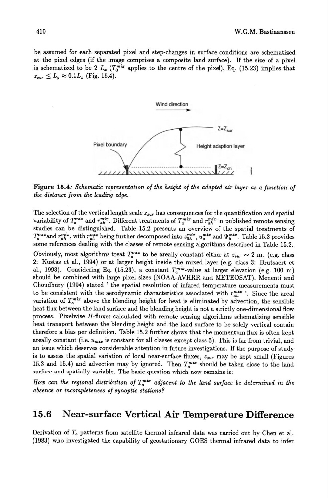
is schematized to be 2 Lx (T;'i'" applies to the centre of the pixel), Eq. (15.23) implies that
Z.ur ::; Ly ~ O.lL", (Fig. 15.4).
Wind direction
Height adaption layer
Figure 15.4: Schematic representation of the height of the adapted air layer as a function of
the distance from the leading edge.
The selection of the vertical length scale Z.ur has consequences for the quantification and spatial
variability of T::i'" and r:;;"'. Different treatments of T::ix and r:;;" in published remote sensing
studies can be distinguished. Table 15.2 presents an overview of the spatial treatments of
T::i"and r:;;", with r:;;" being further decomposed into zgj,ix, u;:'i" and Whix. Table 15.3 provides
some references dealing with the classes of remote sensing algorithms described in Table 15.2.
Obviously, most algorithms treat T::ix to be areally constant either at Z.ur ~ 2 rn. (e.g. class
2: Kustas et aI., 1994) or at larger height inside the mixed layer (e.g. class 3: Brutsaert et
aI., 1993). Considering Eq. (15.23), a constant T::i"-value at larger elevation (e.g. 100 m)
should be combined with large pixel sizes (NOAA-AVHRR and METEOSAT). Menenti and
Choudhury (1994) stated' the spatial resolution of infared temperature measurements must
to be consistent with the aerodynamic characteristics associated with r:;;x '. Since the areal
variation of T::i'" above the blending height for heat is eliminated by advection, the sensible
heat flux between the land surface and the blending height is not a strictly one-dimensional flow
process. Pixelwise H-fluxes calculated with remote sensing algorithms schematizing sensible
heat transport between the blending height and the land surface to be solely vertical contain
therefore a bias per definition. Table 15.2 further shows that the momentum flux is often kept
areally constant (i.e. Urnix is constant for all classes except class 5). This is far from trivial, and
an issue which deserves considerable attention in future investigations. If the purpose of study
is to assess the spatial variation of local near-surface fluxes, Z .ur may be kept small (Figures
15.3 and 15.4) and advection may by ignored. Then T::ix should be taken close to the land
surface and spatially variable. The basic question which now remains is:
How can the regional distribution of T::ix adjacent to the land surface be determined in the
absence or incompleteness of synoptic stations'?
15.6 Near-surface Vertical Air Temperature Difference
Derivation of T.-patterns from satellite thermal infrared data was carried out by Chen et al.
(1983) who investigated the capability of geostationary GOES thermal infrared data to infer
W.G.M. Bastiaanssen
be assumed for each separated pixel and step-changes in surface conditions are schematized
at the pixel edges (if the image comprises a composite land surface). If the size of a pixel
is schematized to be 2 Lx (T;'i'" applies to the centre of the pixel), Eq. (15.23) implies that
Z.ur ::; Ly ~ O.lL", (Fig. 15.4).
Wind direction
Height adaption layer
Figure 15.4: Schematic representation of the height of the adapted air layer as a function of
the distance from the leading edge.
The selection of the vertical length scale Z.ur has consequences for the quantification and spatial
variability of T::i'" and r:;;"'. Different treatments of T::ix and r:;;" in published remote sensing
studies can be distinguished. Table 15.2 presents an overview of the spatial treatments of
T::i"and r:;;", with r:;;" being further decomposed into zgj,ix, u;:'i" and Whix. Table 15.3 provides
some references dealing with the classes of remote sensing algorithms described in Table 15.2.
Obviously, most algorithms treat T::ix to be areally constant either at Z.ur ~ 2 rn. (e.g. class
2: Kustas et aI., 1994) or at larger height inside the mixed layer (e.g. class 3: Brutsaert et
aI., 1993). Considering Eq. (15.23), a constant T::i"-value at larger elevation (e.g. 100 m)
should be combined with large pixel sizes (NOAA-AVHRR and METEOSAT). Menenti and
Choudhury (1994) stated' the spatial resolution of infared temperature measurements must
to be consistent with the aerodynamic characteristics associated with r:;;x '. Since the areal
variation of T::i'" above the blending height for heat is eliminated by advection, the sensible
heat flux between the land surface and the blending height is not a strictly one-dimensional flow
process. Pixelwise H-fluxes calculated with remote sensing algorithms schematizing sensible
heat transport between the blending height and the land surface to be solely vertical contain
therefore a bias per definition. Table 15.2 further shows that the momentum flux is often kept
areally constant (i.e. Urnix is constant for all classes except class 5). This is far from trivial, and
an issue which deserves considerable attention in future investigations. If the purpose of study
is to assess the spatial variation of local near-surface fluxes, Z .ur may be kept small (Figures
15.3 and 15.4) and advection may by ignored. Then T::ix should be taken close to the land
surface and spatially variable. The basic question which now remains is:
How can the regional distribution of T::ix adjacent to the land surface be determined in the
absence or incompleteness of synoptic stations'?
15.6 Near-surface Vertical Air Temperature Difference
Derivation of T.-patterns from satellite thermal infrared data was carried out by Chen et al.
(1983) who investigated the capability of geostationary GOES thermal infrared data to infer