

384
S. Paloscia
of the emissivity and a reduction of the sensitivity to SMC (Choudhury et al., 1979; Wang et
al., 1983).
Since the effect of roughness is dependent on observation wavelength in that a surface can be
rough at 3 cm wavelength and smooth at 21 cm, a multifrequency approach can be useful for
estimating the surface roughness. In general, 10 GHz (3 cm) emission, mainly when measured
at incidence angles higher than 30°, was found to be more sensitive to the soil roughness than
36 GHz (0.8 em) emission, in that the latter saturates as soon as the roughness increases to a
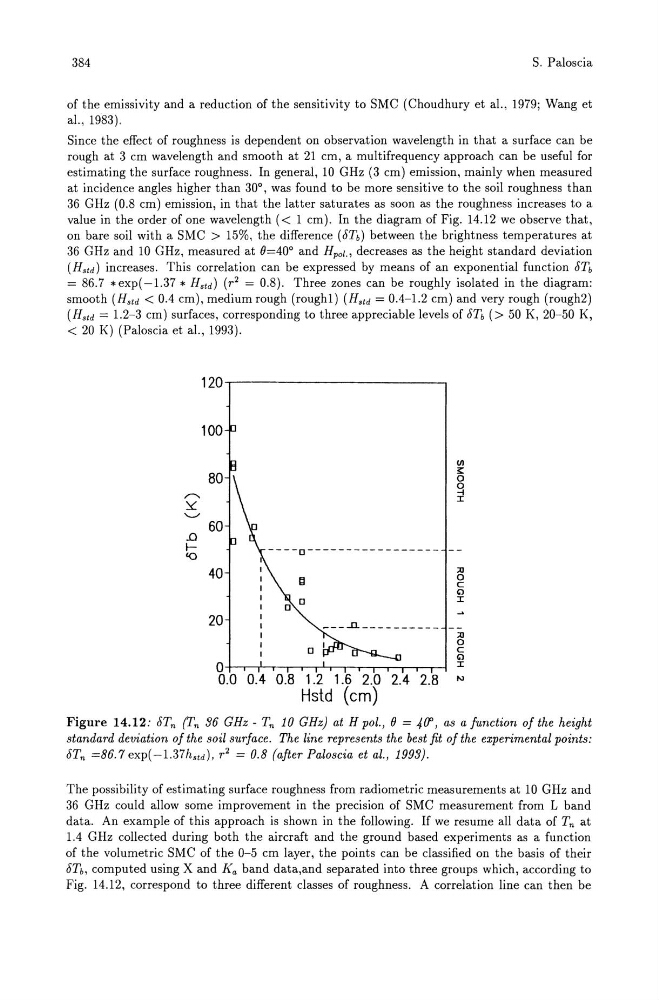
value in the order of one wavelength « 1 cm). In the diagram of Fig. 14.12 we observe that,
on bare soil with a SMC > 15%, the difference (IiTb) between the brightness temperatures at
36 GHz and 10 GHz, measured at 0=40° and Hpol., decreases as the height standard deviation
(Hstd ) increases. This correlation can be expressed by means of an exponential function lin
= 86.7 *exp(-1.37 * Hstd ) (r2 = 0.8). Three zones can be roughly isolated in the diagram:
smooth (Hstd < 0.4 cm), medium rough (roughl) (Hstd = 0.4-1.2 cm) and very rough (rough2)
(Hstd = 1.2-3 cm) surfaces, corresponding to three appreciable levels of lin (> 50 K, 20-50 K,
< 20 K) (Paloscia et al., 1993).
120
100
(11
80
;::
0
0
"
-l
~
I
' - ' 60
.0
----0----------------'0
40
;0
I:l
0
c
(;)
0
I
0
20
___ ..n. __________
;0
0
0
c
(;)
0
I
0.0 0.4 0.8 1.2 1.6 2.0 2.4 2.8 !oJ
Hstd (em)
Figure 14.12: IiTn (Tn 36 GHz· Tn 10 GHz) at Hpol., 0 = 400, as a function of the height
standard deviation of the soil surface. The line represents the best fit of the experimental points:
IiTn =86.1 exp(-1.37h std ) , r2 = 0.8 (afterPaloscia et al., 1993).
The possibility of estimating surface roughness from radiometric measurements at 10 GHz and
36 GHz could allow some improvement in the precision of SMC measurement from L band
data. An example of this approach is shown in the following. If we resume all data of Tn at
1.4 GHz collected during both the aircraft and the ground based experiments as a function
of the volumetric SMC of the 0-5 cm layer, the points can be classified on the basis of their
lin, computed using X and Ka band data,and separated into three groups which, according to
Fig. 14.12, correspond to three different classes of roughness. A correlation line can then be
S. Paloscia
of the emissivity and a reduction of the sensitivity to SMC (Choudhury et al., 1979; Wang et
al., 1983).
Since the effect of roughness is dependent on observation wavelength in that a surface can be
rough at 3 cm wavelength and smooth at 21 cm, a multifrequency approach can be useful for
estimating the surface roughness. In general, 10 GHz (3 cm) emission, mainly when measured
at incidence angles higher than 30°, was found to be more sensitive to the soil roughness than
36 GHz (0.8 em) emission, in that the latter saturates as soon as the roughness increases to a
value in the order of one wavelength « 1 cm). In the diagram of Fig. 14.12 we observe that,
on bare soil with a SMC > 15%, the difference (IiTb) between the brightness temperatures at
36 GHz and 10 GHz, measured at 0=40° and Hpol., decreases as the height standard deviation
(Hstd ) increases. This correlation can be expressed by means of an exponential function lin
= 86.7 *exp(-1.37 * Hstd ) (r2 = 0.8). Three zones can be roughly isolated in the diagram:
smooth (Hstd < 0.4 cm), medium rough (roughl) (Hstd = 0.4-1.2 cm) and very rough (rough2)
(Hstd = 1.2-3 cm) surfaces, corresponding to three appreciable levels of lin (> 50 K, 20-50 K,
< 20 K) (Paloscia et al., 1993).
120
100
(11
80
;::
0
0
"
-l
~
I
' - ' 60
.0
----0----------------'0
40
;0
I:l
0
c
(;)
0
I
0
20
___ ..n. __________
;0
0
0
c
(;)
0
I
0.0 0.4 0.8 1.2 1.6 2.0 2.4 2.8 !oJ
Hstd (em)
Figure 14.12: IiTn (Tn 36 GHz· Tn 10 GHz) at Hpol., 0 = 400, as a function of the height
standard deviation of the soil surface. The line represents the best fit of the experimental points:
IiTn =86.1 exp(-1.37h std ) , r2 = 0.8 (afterPaloscia et al., 1993).
The possibility of estimating surface roughness from radiometric measurements at 10 GHz and
36 GHz could allow some improvement in the precision of SMC measurement from L band
data. An example of this approach is shown in the following. If we resume all data of Tn at
1.4 GHz collected during both the aircraft and the ground based experiments as a function
of the volumetric SMC of the 0-5 cm layer, the points can be classified on the basis of their
lin, computed using X and Ka band data,and separated into three groups which, according to
Fig. 14.12, correspond to three different classes of roughness. A correlation line can then be