

350
Eugene E. Clothiaux, Thomas P. Ackerman, David M. Babb
10 8
10 7
!>. 10 6
.j..l
·rl
fJl
~
Q)
10 5
Cl
H
Q)
~ 10 4
0
p..
10 3
10 2
-0.8
-0.6
-0.4
-0.2
0.0
0.2
Velocity (m 5- 1 )
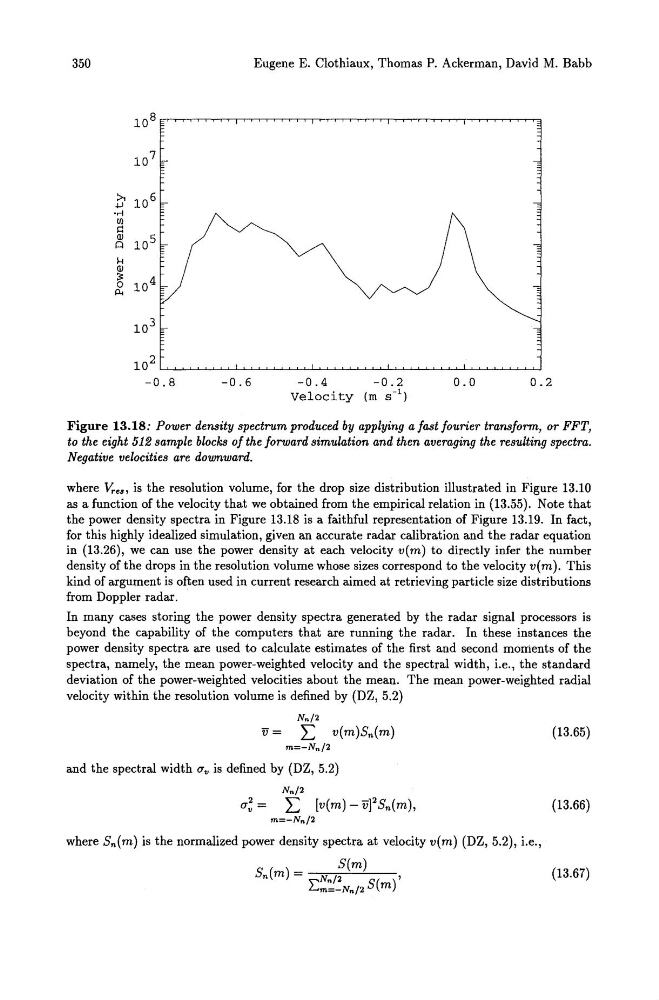
Figure 13.18: Power density spectrum produced by applying a fast fourier transform, or FFT,
to the eight 512 sample blocks of the forward simulation and then averaging the resulting spectra.
Negative velocities are downward.
where Yr • ., is the resolution volume, for the drop size distribution illustrated in Figure 13.10
as a function of the velocity that we obtained from the empirical relation in (13.55). Note that
the power density spectra in Figure 13.18 is a faithful representation of Figure 13.19. In fact,
for this highly idealized simulation, given an accurate radar calibration and the radar equation
in (13.26), we can use the power density at each velocity v(m) to directly infer the number
density of the drops in the resolution volume whose sizes correspond to the velocity v( m). This
kind of argument is often used in current research aimed at retrieving particle size distributions
from Doppler radar.
In many cases storing the power density spectra generated by the radar signal processors is
beyond the capability of the computers that are running the radar. In these instances the
power density spectra are used to calculate estimates of the first and second moments of the
spectra, namely, the mean power-weighted velocity and the spectral width, i.e., the standard
deviation of the power-weighted velocities about the mean. The mean power-weighted radial
velocity within the resolution volume is defined by (DZ, 5.2)
N n /2
V = E v(m)Sn(m)
(13.65)
m=-Nn /2
and the spectral width O'v is defined by (DZ, 5.2)
Nn /2
0' ; = E [v(m) - V]2Sn(m),
(13.66)
m=-Nn /2
where Sn(m) is the normalized power density spectra at velocity v(m) (DZ, 5.2), i.e.,
S (m) _
S(m)
n
-
"Nn /2
S()'
L.m =-Nn /2
m
(13.67)
Eugene E. Clothiaux, Thomas P. Ackerman, David M. Babb
10 8
10 7
!>. 10 6
.j..l
·rl
fJl
~
Q)
10 5
Cl
H
Q)
~ 10 4
0
p..
10 3
10 2
-0.8
-0.6
-0.4
-0.2
0.0
0.2
Velocity (m 5- 1 )
Figure 13.18: Power density spectrum produced by applying a fast fourier transform, or FFT,
to the eight 512 sample blocks of the forward simulation and then averaging the resulting spectra.
Negative velocities are downward.
where Yr • ., is the resolution volume, for the drop size distribution illustrated in Figure 13.10
as a function of the velocity that we obtained from the empirical relation in (13.55). Note that
the power density spectra in Figure 13.18 is a faithful representation of Figure 13.19. In fact,
for this highly idealized simulation, given an accurate radar calibration and the radar equation
in (13.26), we can use the power density at each velocity v(m) to directly infer the number
density of the drops in the resolution volume whose sizes correspond to the velocity v( m). This
kind of argument is often used in current research aimed at retrieving particle size distributions
from Doppler radar.
In many cases storing the power density spectra generated by the radar signal processors is
beyond the capability of the computers that are running the radar. In these instances the
power density spectra are used to calculate estimates of the first and second moments of the
spectra, namely, the mean power-weighted velocity and the spectral width, i.e., the standard
deviation of the power-weighted velocities about the mean. The mean power-weighted radial
velocity within the resolution volume is defined by (DZ, 5.2)
N n /2
V = E v(m)Sn(m)
(13.65)
m=-Nn /2
and the spectral width O'v is defined by (DZ, 5.2)
Nn /2
0' ; = E [v(m) - V]2Sn(m),
(13.66)
m=-Nn /2
where Sn(m) is the normalized power density spectra at velocity v(m) (DZ, 5.2), i.e.,
S (m) _
S(m)
n
-
"Nn /2
S()'
L.m =-Nn /2
m
(13.67)