

Ground-Based Remote Sensing of Cloud Properties ...
349
13.10) and particle fall velocities (Equation 13.55) that we used to generate them in the first
place. This discussion is intended to be illustrative and by no means describes which technique
works best and under what conditions. For a discussion of these issues, Doviak and Zrnic (DZ,
6.4-6.5) is an excellent starting point.
13.7.1 Power density spectra
Extraction of the power density spectra from the I and Q voltages time series is relatively
straightforward (DZ, 5.1). Both the I and Q time series from Section 13.5 have exactly 4096,
or 2 12 , samples. Since the number of samples is a power of 2, we can use anyone of the
standard complex FFT algorithms to generate the power density spectra from the time series
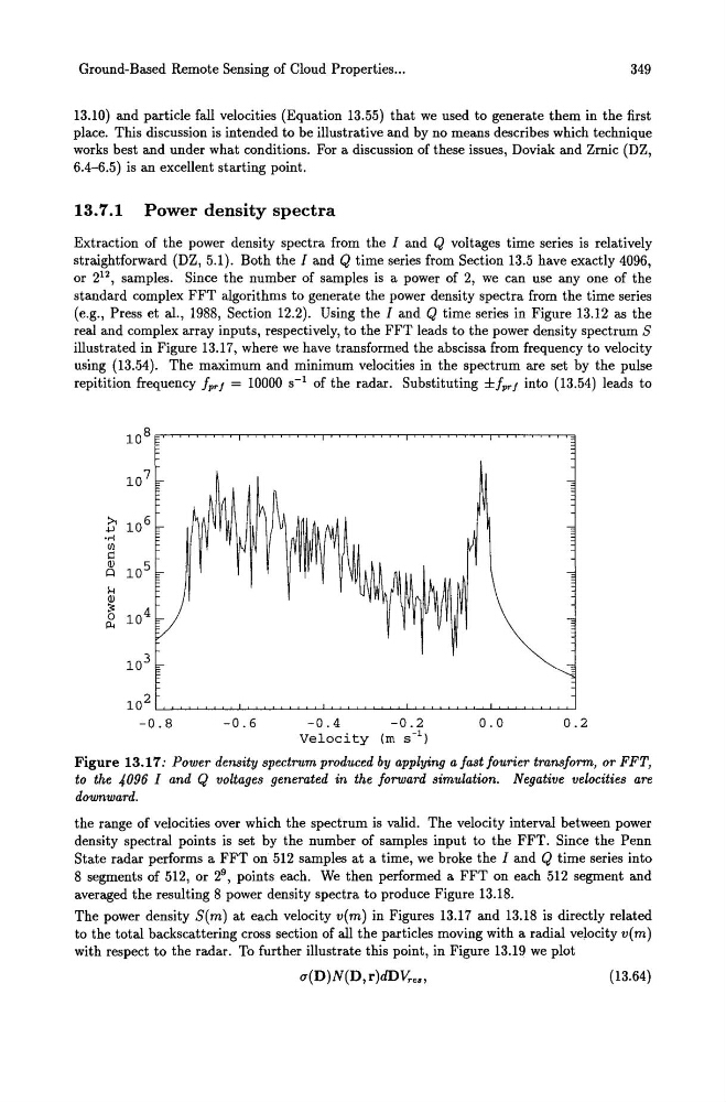
(e.g., Press et al., 1988, Section 12.2). Using the I and Q time series in Figure 13.12 as the
real and complex array inputs, respectively, to the FFT leads to the power density spectrum S
illustrated in Figure 13.17, where we have transformed the abscissa from frequency to velocity
using (13.54). The maximum and minimum velocities in the spectrum are set by the pulse
repitition frequency fprf = 10000 S-l of the radar. Substituting ±fprf into (13.54) leads to
102~~~~~~~~~~~~~~~~~~~~~~~~
-0.8
-0.6
-0.4
-0.2
0.0
0.2
Velocity (m 5- 1 )
Figure 13.17: Power density spectrum produced by applying a fast fourier transform, or FFT,
to the 4096 I and Q voltages generated in the forward simulation. Negative velocities are
downward.
the range of velocities over which the spectrum is valid. The velocity interval between power
density spectral points is set by the number of samples input to the FFT. Since the Penn
State radar performs a FFT on 512 samples at a time, we broke the I and Q time series into
8 segments of 512, or 2 9 , points each. We then performed a FFT on each 512 segment and
averaged the resulting 8 power density spectra to produce Figure 13.18.
The power density SCm) at each velocity v(m) in Figures 13.17 and 13.18 is directly related
to the total backscattering cross section of all the particles moving with a radial velocity v( m)
with respect to the radar. To further illustrate this point, in Figure 13.19 we plot
u(I»N(I>,r)dI)~e.,
(13.64)
349
13.10) and particle fall velocities (Equation 13.55) that we used to generate them in the first
place. This discussion is intended to be illustrative and by no means describes which technique
works best and under what conditions. For a discussion of these issues, Doviak and Zrnic (DZ,
6.4-6.5) is an excellent starting point.
13.7.1 Power density spectra
Extraction of the power density spectra from the I and Q voltages time series is relatively
straightforward (DZ, 5.1). Both the I and Q time series from Section 13.5 have exactly 4096,
or 2 12 , samples. Since the number of samples is a power of 2, we can use anyone of the
standard complex FFT algorithms to generate the power density spectra from the time series
(e.g., Press et al., 1988, Section 12.2). Using the I and Q time series in Figure 13.12 as the
real and complex array inputs, respectively, to the FFT leads to the power density spectrum S
illustrated in Figure 13.17, where we have transformed the abscissa from frequency to velocity
using (13.54). The maximum and minimum velocities in the spectrum are set by the pulse
repitition frequency fprf = 10000 S-l of the radar. Substituting ±fprf into (13.54) leads to
102~~~~~~~~~~~~~~~~~~~~~~~~
-0.8
-0.6
-0.4
-0.2
0.0
0.2
Velocity (m 5- 1 )
Figure 13.17: Power density spectrum produced by applying a fast fourier transform, or FFT,
to the 4096 I and Q voltages generated in the forward simulation. Negative velocities are
downward.
the range of velocities over which the spectrum is valid. The velocity interval between power
density spectral points is set by the number of samples input to the FFT. Since the Penn
State radar performs a FFT on 512 samples at a time, we broke the I and Q time series into
8 segments of 512, or 2 9 , points each. We then performed a FFT on each 512 segment and
averaged the resulting 8 power density spectra to produce Figure 13.18.
The power density SCm) at each velocity v(m) in Figures 13.17 and 13.18 is directly related
to the total backscattering cross section of all the particles moving with a radial velocity v( m)
with respect to the radar. To further illustrate this point, in Figure 13.19 we plot
u(I»N(I>,r)dI)~e.,
(13.64)