

Ground-Based Remote Sensing of Cloud Properties ...
351
10- 3
10- 4 .-s:: 10- 5 =0
.,-1
.j..l
()
Q) 10- 6 =CIl
Ul
Ul
0 10- 7 =H
u
-~"~"\'
.;\
~
10- 8 =10- 9
-0.8
-0.6
-0.4
-0.2
0.0
0.2
Velocity (m 5- 1 )
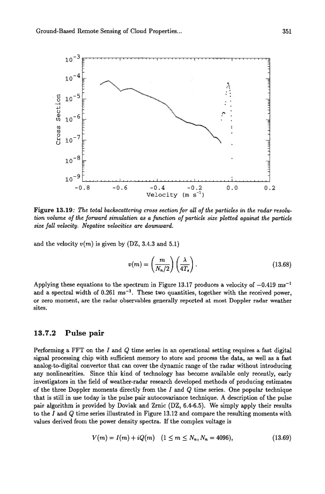
Figure 13.19: The total backscattering cross section for all of the particles in the radar resolution volume of the forward simulation as a function of particle size plotted against the particle
size fall velocity. Negative velocities are downward.
and the velocity v(m) is given by (DZ, 3.4.3 and 5.1)
v(m) = (N~2) (4~J·
(13.68)
Applying these equations to the spectrum in Figure 13.17 produces a velocity of -0.419 ms- I
and a spectral width of 0.261 ms- I . These two quantities, together with the received power,
or zero moment, are the radar observables generally reported at most Doppler radar weather
sites.
13.7.2 Pulse pair
Performing a FFT on the I and Q time series in an operational setting requires a fast digital
signal processing chip with sufficient memory to store and process the data, as well as a fast
analog-to-digital convertor that can cover the dynamic range of the radar without introducing
any nonlinearities. Since this kind of technology has become available only recently, early
investigators in the field of weather-radar research developed methods of producing estimates
of the three Doppler moments directly from the I and Q time series. One popular technique
that is still in use today is the pulse pair autocovariance technique. A description of the pulse
pair algorithm is provided by Doviak and Zrnic (DZ, 6.4-6.5). We simply apply their results
to the I and Q time series illustrated in Figure 13.12 and compare the resulting moments with
values derived from the power density spectra. If the complex voltage is
V(m) = I(m) + iQ(m) (1 ~ m ~ Nn , Nn = 4096),
(13.69)
351
10- 3
10- 4 .-s:: 10- 5 =0
.,-1
.j..l
()
Q) 10- 6 =CIl
Ul
Ul
0 10- 7 =H
u
-~"~"\'
.;\
~
10- 8 =10- 9
-0.8
-0.6
-0.4
-0.2
0.0
0.2
Velocity (m 5- 1 )
Figure 13.19: The total backscattering cross section for all of the particles in the radar resolution volume of the forward simulation as a function of particle size plotted against the particle
size fall velocity. Negative velocities are downward.
and the velocity v(m) is given by (DZ, 3.4.3 and 5.1)
v(m) = (N~2) (4~J·
(13.68)
Applying these equations to the spectrum in Figure 13.17 produces a velocity of -0.419 ms- I
and a spectral width of 0.261 ms- I . These two quantities, together with the received power,
or zero moment, are the radar observables generally reported at most Doppler radar weather
sites.
13.7.2 Pulse pair
Performing a FFT on the I and Q time series in an operational setting requires a fast digital
signal processing chip with sufficient memory to store and process the data, as well as a fast
analog-to-digital convertor that can cover the dynamic range of the radar without introducing
any nonlinearities. Since this kind of technology has become available only recently, early
investigators in the field of weather-radar research developed methods of producing estimates
of the three Doppler moments directly from the I and Q time series. One popular technique
that is still in use today is the pulse pair autocovariance technique. A description of the pulse
pair algorithm is provided by Doviak and Zrnic (DZ, 6.4-6.5). We simply apply their results
to the I and Q time series illustrated in Figure 13.12 and compare the resulting moments with
values derived from the power density spectra. If the complex voltage is
V(m) = I(m) + iQ(m) (1 ~ m ~ Nn , Nn = 4096),
(13.69)