

Ground-Based Remote Sensing of Cloud Properties ...
13.6.2 Signal power statistics
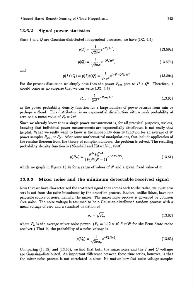
Since I and Q are Gaussian-distributed independent processes, we have (DZ, 4.4)
and
(I) - _1 _ _ [2/2,,2
P - y"i1rcr e
,
(Q) _ _ 1 _ _ Q2/2,,2
P
- y"i1rcr e
,
p(I n Q) = p(I)p(Q) = _1_ e <_[2_Q2)/2,,2
27rcr 2
345
(13.59a)
(13.59b)
(13.59c)
For the present discussion we simply note that the power Pant goes as J2 + Q2. Therefore, it
should come as no surprize that we can write (DZ, 4.4)
(13.60)
as the power probability density function for a large number of power returns from rain or
perhaps a cloud. This distribution is an exponential distribution with a peak probability of
zero and a mean value of Po = 2cr 2 •
Since we already know that a single power measurement is, for all practical purposes, useless,
knowing that individual power measurements are exponentially distributed is not really that
helpful. What we really want to know is the probability density function for an average of N
power samples Pant, or PN . After some mathematical manipulations, that include application of
the residue theorem from the theory of complex numbers, the problem is solved. The resulting
probability density function is (Marshall and Hitschfeld, 1953)
(13.61 )
which we graph in Figure 13.15 for a range of values of N and a given, fixed value of cr.
13.6.3 Mixer noise and the minimum detectable received signal
Now that we have characterized the scattered signal that comes back to the radar, we must now
sort it out from the noise introduced by the detection process. Radars, unlike lidars, have one
principle source of noise, namely, the mixer. The mixer noise process is governed by Johnson
shot noise. The noise voltage is assumed to be a Gaussian-distributed random process with a
mean voltage of zero and a standard deviation of
(13.62)
where Pn is the average mixer noise power. (Pn = 1.12 X 10- 9 mW for the Penn State radar
receiver.) That is, the probability of a noise voltage is
P(Vn) = __ 1_e-v.u2"~.
y"i1rcrv
(13.63)
Comparing (13.59) and (13.63), we find that both the mixer noise and the I and Q voltages
are Gaussian-distributed. An important difference between these time series, however, is that
the mixer noise process is not correlated in time. No matter how fast noise voltage samples
13.6.2 Signal power statistics
Since I and Q are Gaussian-distributed independent processes, we have (DZ, 4.4)
and
(I) - _1 _ _ [2/2,,2
P - y"i1rcr e
,
(Q) _ _ 1 _ _ Q2/2,,2
P
- y"i1rcr e
,
p(I n Q) = p(I)p(Q) = _1_ e <_[2_Q2)/2,,2
27rcr 2
345
(13.59a)
(13.59b)
(13.59c)
For the present discussion we simply note that the power Pant goes as J2 + Q2. Therefore, it
should come as no surprize that we can write (DZ, 4.4)
(13.60)
as the power probability density function for a large number of power returns from rain or
perhaps a cloud. This distribution is an exponential distribution with a peak probability of
zero and a mean value of Po = 2cr 2 •
Since we already know that a single power measurement is, for all practical purposes, useless,
knowing that individual power measurements are exponentially distributed is not really that
helpful. What we really want to know is the probability density function for an average of N
power samples Pant, or PN . After some mathematical manipulations, that include application of
the residue theorem from the theory of complex numbers, the problem is solved. The resulting
probability density function is (Marshall and Hitschfeld, 1953)
(13.61 )
which we graph in Figure 13.15 for a range of values of N and a given, fixed value of cr.
13.6.3 Mixer noise and the minimum detectable received signal
Now that we have characterized the scattered signal that comes back to the radar, we must now
sort it out from the noise introduced by the detection process. Radars, unlike lidars, have one
principle source of noise, namely, the mixer. The mixer noise process is governed by Johnson
shot noise. The noise voltage is assumed to be a Gaussian-distributed random process with a
mean voltage of zero and a standard deviation of
(13.62)
where Pn is the average mixer noise power. (Pn = 1.12 X 10- 9 mW for the Penn State radar
receiver.) That is, the probability of a noise voltage is
P(Vn) = __ 1_e-v.u2"~.
y"i1rcrv
(13.63)
Comparing (13.59) and (13.63), we find that both the mixer noise and the I and Q voltages
are Gaussian-distributed. An important difference between these time series, however, is that
the mixer noise process is not correlated in time. No matter how fast noise voltage samples