

344
Eugene E. Clothiaux, Thomas P. Ackerman, David M. Babb
I are obtained in a vanishingly short period of time, their values converge. (In Figure 13.12
neighboring I voltages in time are always similar in magnitude.) Knowing I at one instant
does provide some useful information in figuring out the values of I at later not to far in the
distant future times. The autocorrelation function defined by
(13.57)
provides a quantitative assessment of how the I voltages are correlated when offset by a lag of
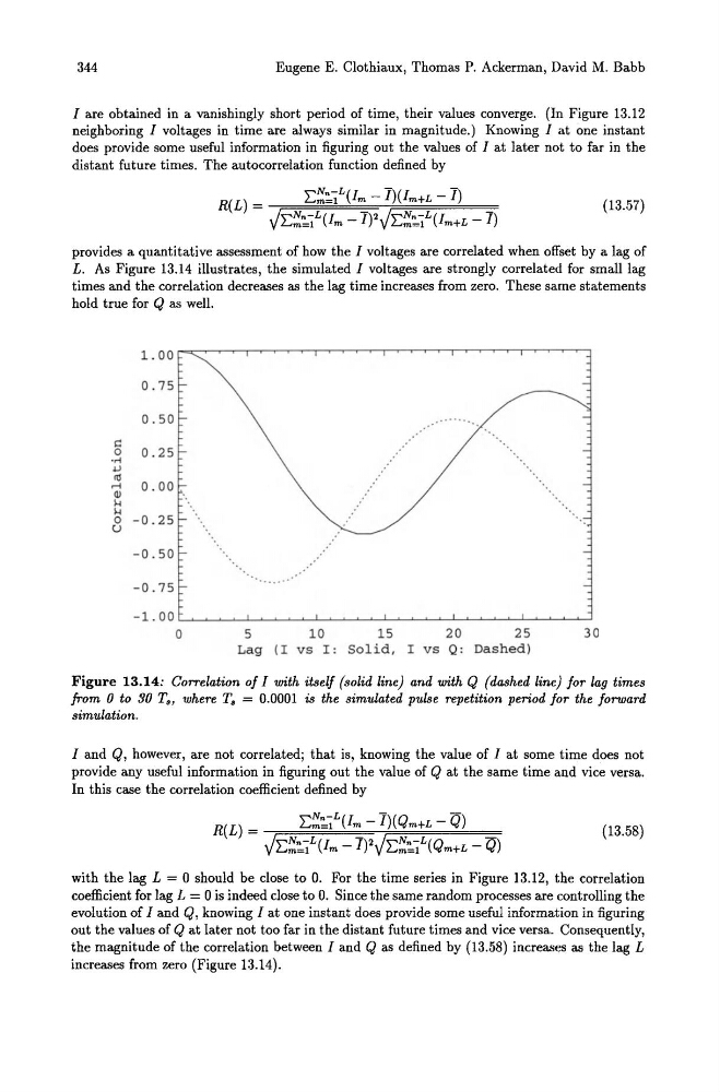
L. As Figure 13.14 illustrates, the simulated I voltages are strongly correlated for small lag
times and the correlation decreases as the lag time increases from zero. These same statements
hold true for Q as well.
1. 00
0.75
0.50
f;!
0
'M
0.25
~
nJ
r-l
Q)
0.00
...
... 0
u
- 0.25
- 0.50
.'
-0.75
-1 . 00
0
5
10
15
20
25
30
Lag (I vs I: Solid, I vs Q: Dashed)
Figure 13.14: Correlation of I with itself (solid line) and with Q (dashed line) for lag times
from 0 to 30 To, where T. = 0.0001 is the simulated pulse repetition period for the forward
simulation.
I and Q, however, are not correlated; that is, knowing the value of I at some time does not
provide any useful information in figuring out the value of Q at the same time and vice versa.
In this case the correlation coefficient defined by
(13.58)
with the lag L = 0 should be close to O. For the time series in Figure 13.12, the correlation
coefficient for lag L = 0 is indeed close to O. Since the same random processes are controlling the
evolution of I and Q, knowing I at one instant does provide some useful information in figuring
out the values of Q at later not too far in the distant future times and vice versa. Consequently,
the magnitude of the correlation between I and Q as defined by (13.58) increases as the lag L
increases from zero (Figure 13.14).
Eugene E. Clothiaux, Thomas P. Ackerman, David M. Babb
I are obtained in a vanishingly short period of time, their values converge. (In Figure 13.12
neighboring I voltages in time are always similar in magnitude.) Knowing I at one instant
does provide some useful information in figuring out the values of I at later not to far in the
distant future times. The autocorrelation function defined by
(13.57)
provides a quantitative assessment of how the I voltages are correlated when offset by a lag of
L. As Figure 13.14 illustrates, the simulated I voltages are strongly correlated for small lag
times and the correlation decreases as the lag time increases from zero. These same statements
hold true for Q as well.
1. 00
0.75
0.50
f;!
0
'M
0.25
~
nJ
r-l
Q)
0.00
...
... 0
u
- 0.25
- 0.50
.'
-0.75
-1 . 00
0
5
10
15
20
25
30
Lag (I vs I: Solid, I vs Q: Dashed)
Figure 13.14: Correlation of I with itself (solid line) and with Q (dashed line) for lag times
from 0 to 30 To, where T. = 0.0001 is the simulated pulse repetition period for the forward
simulation.
I and Q, however, are not correlated; that is, knowing the value of I at some time does not
provide any useful information in figuring out the value of Q at the same time and vice versa.
In this case the correlation coefficient defined by
(13.58)
with the lag L = 0 should be close to O. For the time series in Figure 13.12, the correlation
coefficient for lag L = 0 is indeed close to O. Since the same random processes are controlling the
evolution of I and Q, knowing I at one instant does provide some useful information in figuring
out the values of Q at later not too far in the distant future times and vice versa. Consequently,
the magnitude of the correlation between I and Q as defined by (13.58) increases as the lag L
increases from zero (Figure 13.14).