

340
Eugene E. Clothiaux, Thomas P. Ackerman, David M. Babb
13.5 An Example
Before discussing the properties of the I and Q voltages, as well as the Doppler moments, we
thought that it would be instructive to illustrate all of the previous discussion with a realistic,
but computer simulated, "meteorological target". To this end we illustrate the results of a forward computer simulation in which we explicity calculate the I and Q voltages for a specified
drop size distribution located within a specified resolution volume. In situ measurements by
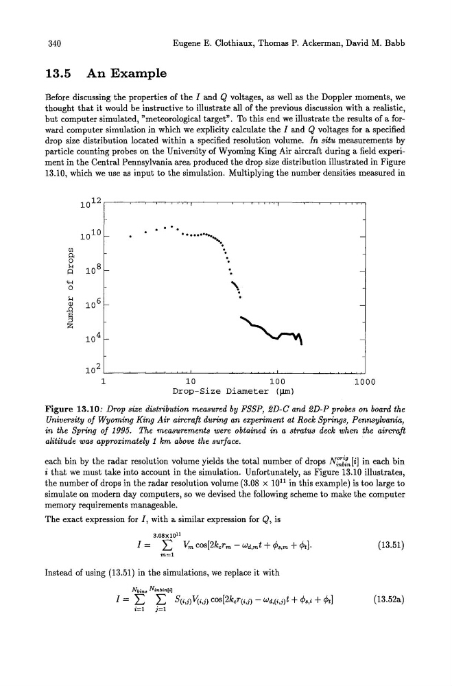
particle counting probes on the University of Wyoming King Air aircraft during a field experiment in the Central Pennsylvania area produced the drop size distribution illustrated in Figure
13.10, which we use as input to the simulation. Multiplying the number densities measured in
10 12
10 10 -
................
-
. . ..
Ul
0.
0
..
..
H
10 8 -
Q
..
-
~
0
\
H
10 6 -
Q)
il
-
;:::s
Z
10 4 -
-
10 2
1
10
100
1000
Drop-Size Diameter (~)
Figure 13.10: Drop size distribution measured by FSSP, 2D-C and 2D-P probes on board the
University of Wyoming King Air aircraft during an experiment at Rock Springs, Pennsylvania,
in the Spring of 1995. The measurements were obtained in a stratus deck when the aircraft
alititude was approximately 1 km above the surface.
each bin by the radar resolution volume yields the total number of drops N:;~!n[il in each bin
i that we must take into account in the simulation. Unfortunately, as Figure 13.10 illustrates,
the number of drops in the radar resolution volume (3.08 x 10¹¹ in this example) is too large to
simulate on modern day computers, so we devised the following scheme to make the computer
memory requirements manageable.
The exact expression for I, with a similar expression for Q, is
3.08X10"
1= L Vm cos[2kcrm - Wd,m t + cPs,m + cPtl·
(13.51 )
m=l
Instead of using (13.51) in the simulations, we replace it with
NbintJ Ninbin[i]
I = L L S(i,j) Vii,j) cos[2kcr(i,j) - Wd,(i,jJt + cPs,i + cPtl
(13.52a)
i=l
j=l
Eugene E. Clothiaux, Thomas P. Ackerman, David M. Babb
13.5 An Example
Before discussing the properties of the I and Q voltages, as well as the Doppler moments, we
thought that it would be instructive to illustrate all of the previous discussion with a realistic,
but computer simulated, "meteorological target". To this end we illustrate the results of a forward computer simulation in which we explicity calculate the I and Q voltages for a specified
drop size distribution located within a specified resolution volume. In situ measurements by
particle counting probes on the University of Wyoming King Air aircraft during a field experiment in the Central Pennsylvania area produced the drop size distribution illustrated in Figure
13.10, which we use as input to the simulation. Multiplying the number densities measured in
10 12
10 10 -
................
-
. . ..
Ul
0.
0
..
..
H
10 8 -
Q
..
-
~
0
\
H
10 6 -
Q)
il
-
;:::s
Z
10 4 -
-
10 2
1
10
100
1000
Drop-Size Diameter (~)
Figure 13.10: Drop size distribution measured by FSSP, 2D-C and 2D-P probes on board the
University of Wyoming King Air aircraft during an experiment at Rock Springs, Pennsylvania,
in the Spring of 1995. The measurements were obtained in a stratus deck when the aircraft
alititude was approximately 1 km above the surface.
each bin by the radar resolution volume yields the total number of drops N:;~!n[il in each bin
i that we must take into account in the simulation. Unfortunately, as Figure 13.10 illustrates,
the number of drops in the radar resolution volume (3.08 x 10¹¹ in this example) is too large to
simulate on modern day computers, so we devised the following scheme to make the computer
memory requirements manageable.
The exact expression for I, with a similar expression for Q, is
3.08X10"
1= L Vm cos[2kcrm - Wd,m t + cPs,m + cPtl·
(13.51 )
m=l
Instead of using (13.51) in the simulations, we replace it with
NbintJ Ninbin[i]
I = L L S(i,j) Vii,j) cos[2kcr(i,j) - Wd,(i,jJt + cPs,i + cPtl
(13.52a)
i=l
j=l