

Ground-Based Remote Sensing of Cloud Properties ...
339
if Pant is measured repeatedly over a time interval long compared with the time intervals
27r/(Wd,m -Wd,n),m # n, and averaged, the second sum does indeed go to zero. Therefore, we
can write
[
1 N n
]
1 N.
Pant = Nlim -N L Pant,j = -2 L (A:")\
"-+00
n j=1
"70 m=l
(13.45)
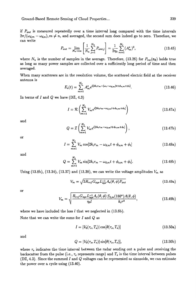
where Nn is the number of samples in the average. Therefore, (13.26) for Prec(ro) holds true
as long as many power samples are collected over a sufficiently long period of time and then
averaged.
When many scatterers are in the resolution volume, the scattered electric field at the receiver
antenna is
N.
Es(t) = L A:"ei[2k,rm-(w,-Wd,m)t+
m=l
In terms of I and Q we have (DZ, 4.3)
1= R.. (~ Vmei[2k,rm-wd,mt+
(13.47a)
and
Q = I (~ Vmei[2k,rm-wd,mt+
(13.47b)
or
N.
I = L Vm cos[2kcrm - Wd,mt +
m=l
and
N.
Q = L Vm sin[2kcr m - Wd,mt +
m=l
Using (13.8b), (13.34), (13.37) and (13.38), we can write the voltage amplitudes Vm as
or
where we have included the loss l that we neglected in (13.8b).
Note that we can write the sums for I and Q as
1= I Vo(r., T.)I cos [O(r., T.))
and
Q = IVo(r.,T.)lsin[O(r.,T.)),
(13.49a)
(13.49b)
(13.50a)
(13.50b)
where rs indicates the time interval between the radar sending out a pulse and receiving the
backscatter from the pulse (i.e., rs represents range) and Ts is the time interval between pulses
(DZ,4.3). Since the summed I and Q voltages can be represented as sinusoids, we can estimate
the power over a cycle using (13.40).
339
if Pant is measured repeatedly over a time interval long compared with the time intervals
27r/(Wd,m -Wd,n),m # n, and averaged, the second sum does indeed go to zero. Therefore, we
can write
[
1 N n
]
1 N.
Pant = Nlim -N L Pant,j = -2 L (A:")\
"-+00
n j=1
"70 m=l
(13.45)
where Nn is the number of samples in the average. Therefore, (13.26) for Prec(ro) holds true
as long as many power samples are collected over a sufficiently long period of time and then
averaged.
When many scatterers are in the resolution volume, the scattered electric field at the receiver
antenna is
N.
Es(t) = L A:"ei[2k,rm-(w,-Wd,m)t+
m=l
In terms of I and Q we have (DZ, 4.3)
1= R.. (~ Vmei[2k,rm-wd,mt+
(13.47a)
and
Q = I (~ Vmei[2k,rm-wd,mt+
(13.47b)
or
N.
I = L Vm cos[2kcrm - Wd,mt +
m=l
and
N.
Q = L Vm sin[2kcr m - Wd,mt +
m=l
Using (13.8b), (13.34), (13.37) and (13.38), we can write the voltage amplitudes Vm as
or
where we have included the loss l that we neglected in (13.8b).
Note that we can write the sums for I and Q as
1= I Vo(r., T.)I cos [O(r., T.))
and
Q = IVo(r.,T.)lsin[O(r.,T.)),
(13.49a)
(13.49b)
(13.50a)
(13.50b)
where rs indicates the time interval between the radar sending out a pulse and receiving the
backscatter from the pulse (i.e., rs represents range) and Ts is the time interval between pulses
(DZ,4.3). Since the summed I and Q voltages can be represented as sinusoids, we can estimate
the power over a cycle using (13.40).