

338
Eugene E. Clothiaux, Thomas P. Ackerman, David M. Babb
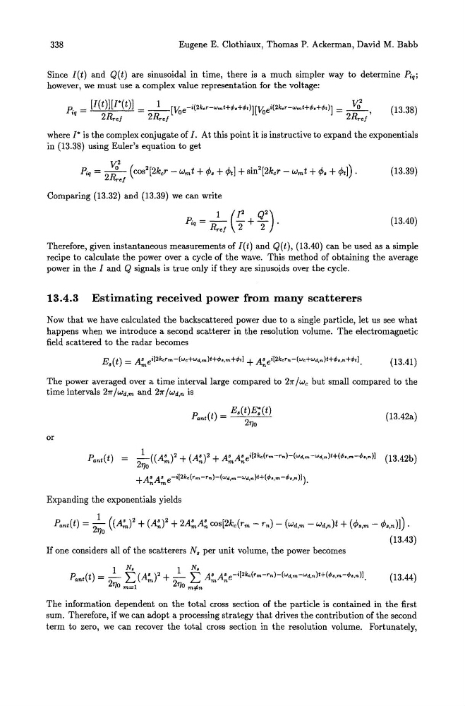
Since l(t) and Q(t) are sinusoidal in time, there is a much simpler way to determine Pjq ;
however, we must use a complex value representation for the voltage:
(13.38)
where 1* is the complex conjugate of I. At this point it is instructive to expand the exponentials
in (13.38) using Euler's equation to get
Pjq = ~2 (cos2[2kcr _ wmt +
Comparing (13.32) and (13.39) we can write
p.- = _1_ (12 + Q2)
.q
Rref
2
2 .
(13.39)
(13.40)
Therefore, given instantaneous measurements of l(t) and Q(t), (13.40) can be used as a simple
recipe to calculate the power over a cycle of the wave. This method of obtaining the average
power in the I and Q signals is true only if they are sinusoids over the cycle.
13.4.3 Estimating received power from many scatterers
Now that we have calculated the backscattered power due to a single particle, let us see what
happens when we introduce a second scatterer in the resolution volume. The electromagnetic
field scattered to the radar becomes
(13.41 )
The power averaged over a time interval large compared to 271" /wc but small compared to the
time intervals 271" / Wd,m and 271" / Wd,n is
or
p. () _ Es(t)E;(t)
ant t - --'-":"2"-"-'--'7]0
(13.42a)
2~0 ((A:'Y + (A~)2 + A:"A~ei[2ke(r,n-rn)-(Wd,m-Wd,n)t+(q,.,m-q,.,n)] (13.42b)
+ A~A:" e- j [2ke(rm-rn )-(Wd,m -Wd,n)t+(q,.,m-q,.,n)]).
Expanding the exponentials yields
Pant(t) = 2~0 ((A:,,)2 + (A~)2 + 2A:"A~ cos[2kc(rm - rn) - (Wd,m - Wd,n)t + (
If one considers all of the scatterers N. per unit volume, the power becomes
(13.44)
The information dependent on the total cross section of the particle is contained in the first
sum. Therefore, if we can adopt a processing strategy that drives the contribution of the second
term to zero, we can recover the total cross section in the resolution volume. Fortunately,
Eugene E. Clothiaux, Thomas P. Ackerman, David M. Babb
Since l(t) and Q(t) are sinusoidal in time, there is a much simpler way to determine Pjq ;
however, we must use a complex value representation for the voltage:
(13.38)
where 1* is the complex conjugate of I. At this point it is instructive to expand the exponentials
in (13.38) using Euler's equation to get
Pjq = ~2 (cos2[2kcr _ wmt +
Comparing (13.32) and (13.39) we can write
p.- = _1_ (12 + Q2)
.q
Rref
2
2 .
(13.39)
(13.40)
Therefore, given instantaneous measurements of l(t) and Q(t), (13.40) can be used as a simple
recipe to calculate the power over a cycle of the wave. This method of obtaining the average
power in the I and Q signals is true only if they are sinusoids over the cycle.
13.4.3 Estimating received power from many scatterers
Now that we have calculated the backscattered power due to a single particle, let us see what
happens when we introduce a second scatterer in the resolution volume. The electromagnetic
field scattered to the radar becomes
(13.41 )
The power averaged over a time interval large compared to 271" /wc but small compared to the
time intervals 271" / Wd,m and 271" / Wd,n is
or
p. () _ Es(t)E;(t)
ant t - --'-":"2"-"-'--'7]0
(13.42a)
2~0 ((A:'Y + (A~)2 + A:"A~ei[2ke(r,n-rn)-(Wd,m-Wd,n)t+(q,.,m-q,.,n)] (13.42b)
+ A~A:" e- j [2ke(rm-rn )-(Wd,m -Wd,n)t+(q,.,m-q,.,n)]).
Expanding the exponentials yields
Pant(t) = 2~0 ((A:,,)2 + (A~)2 + 2A:"A~ cos[2kc(rm - rn) - (Wd,m - Wd,n)t + (
If one considers all of the scatterers N. per unit volume, the power becomes
(13.44)
The information dependent on the total cross section of the particle is contained in the first
sum. Therefore, if we can adopt a processing strategy that drives the contribution of the second
term to zero, we can recover the total cross section in the resolution volume. Fortunately,