

334
Eugene E. Clothiaux, Thomas P. Ackerman, David M. Babb
il~-----------~-- I
~ Distance
o
c to
(a)
I
C1-. ~ Distance
o
cto
(b)
-: -1- 1-: Distance
I
c to
(c)
o
-p
I
~ Distance
o
C to
(d)
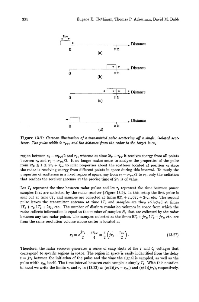
Figure 13.7: Cartoon illustration of a transmitted pulse scattering off a single, isolated scatterer. The pulse width is Tpw, and the distance /rom the radar to the target is eto.
region between ro - CTpw /2 and ro, whereas at time 2to + Tpw it receives energy from all points
between ro and ro + cTpw /2. It no longer makes sense to analyze the properties of the pulse
from 2to :s t :s 2to + Tpw to infer properties about the scatterer located at position ro since
the radar is receiving energy from different points in space during this interval. To study the
properties of scatterers in a fixed region of space, say from ro - CTpw/2 to ro, only the radiation
that reaches the receiver antenna at the precise time of 2to is of value.
Let T. represent the time between radar pulses and let T. represent the time between power
samples that are collected by the radar receiver (Figure 13.9). In this setup the first pulse is
sent out at time QT. and samples are collected at times QT. + T., QT. + 2T., etc. The second
pulse leaves the transmitter antenna at time IT. and samples are then collected at times
IT. + T., IT. + 2T., etc. The number of distinct resolution volumes in space from which the
radar collects information is equal to the number of samples Ng that are collected by the radar
between any two radar pulses. The samples collected at the times QT. + jT., IT. + jT., etc. are
from the same resolution volume whose center is located at
(13.27)
Therefore, the radar receiver generates a series of snap shots of the I and Q voltages that
correspond to specific regions in space. The region in space is easily indentified from the delay
t = jT. between the initiation of the pulse and the time the signal is sampled, as well as the
pulse width Tpw itself. The time interval between each sample is simply T •. With this notation
in hand we write the limits rb and rt in (13.23) as (C/2)(jT. - Tpw) and (C/2)(jT.), respectively.
Eugene E. Clothiaux, Thomas P. Ackerman, David M. Babb
il~-----------~-- I
~ Distance
o
c to
(a)
I
C1-. ~ Distance
o
cto
(b)
-: -1- 1-: Distance
I
c to
(c)
o
-p
I
~ Distance
o
C to
(d)
Figure 13.7: Cartoon illustration of a transmitted pulse scattering off a single, isolated scatterer. The pulse width is Tpw, and the distance /rom the radar to the target is eto.
region between ro - CTpw /2 and ro, whereas at time 2to + Tpw it receives energy from all points
between ro and ro + cTpw /2. It no longer makes sense to analyze the properties of the pulse
from 2to :s t :s 2to + Tpw to infer properties about the scatterer located at position ro since
the radar is receiving energy from different points in space during this interval. To study the
properties of scatterers in a fixed region of space, say from ro - CTpw/2 to ro, only the radiation
that reaches the receiver antenna at the precise time of 2to is of value.
Let T. represent the time between radar pulses and let T. represent the time between power
samples that are collected by the radar receiver (Figure 13.9). In this setup the first pulse is
sent out at time QT. and samples are collected at times QT. + T., QT. + 2T., etc. The second
pulse leaves the transmitter antenna at time IT. and samples are then collected at times
IT. + T., IT. + 2T., etc. The number of distinct resolution volumes in space from which the
radar collects information is equal to the number of samples Ng that are collected by the radar
between any two radar pulses. The samples collected at the times QT. + jT., IT. + jT., etc. are
from the same resolution volume whose center is located at
(13.27)
Therefore, the radar receiver generates a series of snap shots of the I and Q voltages that
correspond to specific regions in space. The region in space is easily indentified from the delay
t = jT. between the initiation of the pulse and the time the signal is sampled, as well as the
pulse width Tpw itself. The time interval between each sample is simply T •. With this notation
in hand we write the limits rb and rt in (13.23) as (C/2)(jT. - Tpw) and (C/2)(jT.), respectively.