

88
,1,';-- __
~
'11
~,
--~
~--------------- ~------~~,
v,
V,
~
~A\n
V1
V1
V~--_~_--: __ _
---------------------- -------------- ---~~
j~
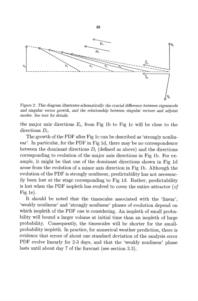
Figure 2: This diagram illustrates schematically the crucial difference between eigenmode
and singular vector growth, and the relationship between singular vectors and adjoint
modes. See text for details.
the major axis directions Ei , from Fig lb to Fig lc will be close to the
directions D i .
The growth of the PDF after Fig lc can be described as 'strongly nonlinear'. In particular, for the PDF in Fig ld, there may be no correspondence
between the dominant directions Di (defined as above) and the directions
corresponding to evolution of the major axis directions in Fig lb. For example, it might be that one of the dominant directions shown in Fig ld
arose from the evolution of a minor axis direction in Fig lb. Although the
evolution of the PDF is strongly nonlinear, predictability has not necessarily been lost at the stage corresponding to Fig ld. Rather, predictability
is lost when the PDF isopleth has evolved to cover the entire attractor (cf
Fig Ie).
It should be noted that the timescales associated with the 'linear',
'weakly nonlinear' and 'strongly nonlinear' phases of evolution depend on
which isopleth of the PDF one is considering. An isopleth of small probability will bound a larger volume at initial time than an isopleth of large
probability. Consequently, the timescales will be shorter for the smallprobability isopleth. In practice, for numerical weather prediction, there is
evidence that errors of about one standard deviation of the analysis error
PDF evolve linearly for 2-3 days, and that the 'weakly nonlinear' phase
lasts until about day 7 of the forecast (see section 3.3).
,1,';-- __
~
'11
~,
--~
~--------------- ~------~~,
v,
V,
~
~A\n
V1
V1
V~--_~_--: __ _
---------------------- -------------- ---~~
j~
Figure 2: This diagram illustrates schematically the crucial difference between eigenmode
and singular vector growth, and the relationship between singular vectors and adjoint
modes. See text for details.
the major axis directions Ei , from Fig lb to Fig lc will be close to the
directions D i .
The growth of the PDF after Fig lc can be described as 'strongly nonlinear'. In particular, for the PDF in Fig ld, there may be no correspondence
between the dominant directions Di (defined as above) and the directions
corresponding to evolution of the major axis directions in Fig lb. For example, it might be that one of the dominant directions shown in Fig ld
arose from the evolution of a minor axis direction in Fig lb. Although the
evolution of the PDF is strongly nonlinear, predictability has not necessarily been lost at the stage corresponding to Fig ld. Rather, predictability
is lost when the PDF isopleth has evolved to cover the entire attractor (cf
Fig Ie).
It should be noted that the timescales associated with the 'linear',
'weakly nonlinear' and 'strongly nonlinear' phases of evolution depend on
which isopleth of the PDF one is considering. An isopleth of small probability will bound a larger volume at initial time than an isopleth of large
probability. Consequently, the timescales will be shorter for the smallprobability isopleth. In practice, for numerical weather prediction, there is
evidence that errors of about one standard deviation of the analysis error
PDF evolve linearly for 2-3 days, and that the 'weakly nonlinear' phase
lasts until about day 7 of the forecast (see section 3.3).