

54
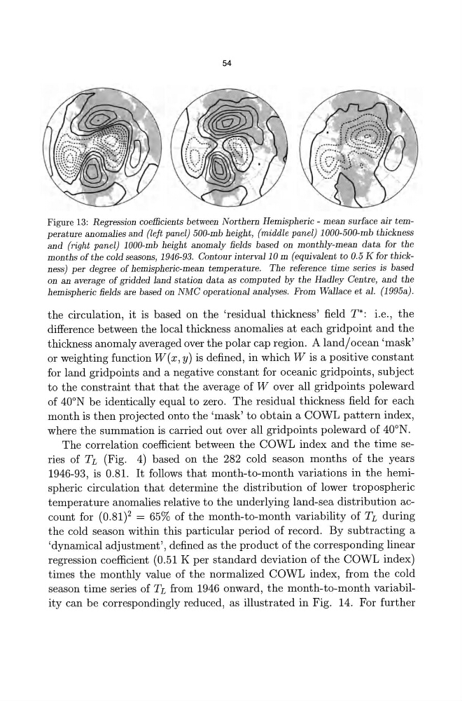
Figure 13: Regression coeiHcients between Northern Hemispheric - mean surface air temperature anomalies and (left panel) 500-mb height, (middle panel) 1000-500-mb thickness
and (right panel) 1000-mb height anomaly fields based on monthly-mean data for the
months of the cold seasons, 1946-93. Contour interval 10 m (equivalent to 0.5 K for thickness) per degree of hemispheric-mean temperature. The reference time series is based
on an average of gridded land station data as computed by the Hadley Centre, and the
hemispheric fields are based on NMC operational analyses. From Wallace et al. (1995a) .
the circulation, it is based on the 'residual thickness' field T*: i.e., the
difference between the local thickness anomalies at each gridpoint and the
thickness anomaly averaged over the polar cap region. A land/ocean 'mask'
or weighting function W(x, y) is defined, in which W is a positive constant
for land gridpoints and a negative constant for oceanic gridpoints, subject
to the constraint that that the average of W over all gridpoints poleward
of 400N be identically equal to zero. The residual thickness field for each
month is then projected onto the 'mask' to obtain a COWL pattern index,
where the summation is carried out over all gridpoints poleward of 40oN.
The correlation coefficient between the COWL index and the time series of TL (Fig. 4) based on the 282 cold season months of the years
1946-93, is 0.81. It follows that month-to-month variations in the hemispheric circulation that determine the distribution of lower tropospheric
temperature anomalies relative to the underlying land-sea distribution account for (0.81)2 = 65% of the month-to-month variability of TL during
the cold season within this particular period of record. By subtracting a
'dynamical adjustment' , defined as the product of the corresponding linear
regression coefficient (0.51 K per standard deviation of the COWL index)
times the monthly value of the normalized COWL index, from the cold
season time series of TL from 1946 onward, the month-to-month variability can be correspondingly reduced, as illustrated in Fig. 14. For further
Figure 13: Regression coeiHcients between Northern Hemispheric - mean surface air temperature anomalies and (left panel) 500-mb height, (middle panel) 1000-500-mb thickness
and (right panel) 1000-mb height anomaly fields based on monthly-mean data for the
months of the cold seasons, 1946-93. Contour interval 10 m (equivalent to 0.5 K for thickness) per degree of hemispheric-mean temperature. The reference time series is based
on an average of gridded land station data as computed by the Hadley Centre, and the
hemispheric fields are based on NMC operational analyses. From Wallace et al. (1995a) .
the circulation, it is based on the 'residual thickness' field T*: i.e., the
difference between the local thickness anomalies at each gridpoint and the
thickness anomaly averaged over the polar cap region. A land/ocean 'mask'
or weighting function W(x, y) is defined, in which W is a positive constant
for land gridpoints and a negative constant for oceanic gridpoints, subject
to the constraint that that the average of W over all gridpoints poleward
of 400N be identically equal to zero. The residual thickness field for each
month is then projected onto the 'mask' to obtain a COWL pattern index,
where the summation is carried out over all gridpoints poleward of 40oN.
The correlation coefficient between the COWL index and the time series of TL (Fig. 4) based on the 282 cold season months of the years
1946-93, is 0.81. It follows that month-to-month variations in the hemispheric circulation that determine the distribution of lower tropospheric
temperature anomalies relative to the underlying land-sea distribution account for (0.81)2 = 65% of the month-to-month variability of TL during
the cold season within this particular period of record. By subtracting a
'dynamical adjustment' , defined as the product of the corresponding linear
regression coefficient (0.51 K per standard deviation of the COWL index)
times the monthly value of the normalized COWL index, from the cold
season time series of TL from 1946 onward, the month-to-month variability can be correspondingly reduced, as illustrated in Fig. 14. For further