

463
,:"",
/'"
...... :,
0.0
0.1
0.2
0.3
0.4
0.5
Frequency (cycles/months)
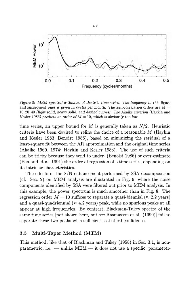
Figure 8: MEM spectral estimates of the SOl time series. The frequency in this figure
and subsequent ones is given in cycles per month. The autocorrelation orders are M =
10 , 20 ,40 (light solid, heavy solid, and dashed curves). The Akaike criterion (Haykin and
Kesler 1983) predicts an order of M ::::: 10, which is obviously too low.
time series, an upper bound for M is generally taken as N 12. Heuristic
criteria have been devised to refine the choice of a reasonable M (Haykin
and Kesler 1983, Benoist 1986), based on minimizing the residual of a
least-square fit between the AR approximation and the original time series
(Akaike 1969, 1974; Haykin and Kesler 1983). The use of such criteria
can be tricky because they tend to under- (Benoist 1986) or over-estimate
(Penland et al. 1991) the order of regression of a time series, depending on
its intrinsic characteristics.
The effects of the S IN enhancement performed by SSA decomposition
(cf. Sec. 2) on MEM analysis are illustrated in Fig. 9, where the noise
components identified by SSA were filtered out prior to MEM analysis. In
this example, the power spectrum is much smoother than in Fig. 8. The
regression order M = 10 suffices to separate a quasi-biennial (~ 2.2 years)
and a quasi-quadriennial (~ 4.2 years) peak, while no spurious peaks at all
appear at high frequencies . By contrast, Blackman-Tukey spectra of the
same time series [not shown here, but see Rasmusson et al. (1990)] fail to
separate these two peaks with sufficient statistical confidence.
3.3 Multi-Taper Method (MTM)
This method, like that of Blackman and Thkey (1958) in Sec. 3.1, is nonparametric, i.e. - unlike MEM - it does not use a specific, parameter-
,:"",
/'"
...... :,
0.0
0.1
0.2
0.3
0.4
0.5
Frequency (cycles/months)
Figure 8: MEM spectral estimates of the SOl time series. The frequency in this figure
and subsequent ones is given in cycles per month. The autocorrelation orders are M =
10 , 20 ,40 (light solid, heavy solid, and dashed curves). The Akaike criterion (Haykin and
Kesler 1983) predicts an order of M ::::: 10, which is obviously too low.
time series, an upper bound for M is generally taken as N 12. Heuristic
criteria have been devised to refine the choice of a reasonable M (Haykin
and Kesler 1983, Benoist 1986), based on minimizing the residual of a
least-square fit between the AR approximation and the original time series
(Akaike 1969, 1974; Haykin and Kesler 1983). The use of such criteria
can be tricky because they tend to under- (Benoist 1986) or over-estimate
(Penland et al. 1991) the order of regression of a time series, depending on
its intrinsic characteristics.
The effects of the S IN enhancement performed by SSA decomposition
(cf. Sec. 2) on MEM analysis are illustrated in Fig. 9, where the noise
components identified by SSA were filtered out prior to MEM analysis. In
this example, the power spectrum is much smoother than in Fig. 8. The
regression order M = 10 suffices to separate a quasi-biennial (~ 2.2 years)
and a quasi-quadriennial (~ 4.2 years) peak, while no spurious peaks at all
appear at high frequencies . By contrast, Blackman-Tukey spectra of the
same time series [not shown here, but see Rasmusson et al. (1990)] fail to
separate these two peaks with sufficient statistical confidence.
3.3 Multi-Taper Method (MTM)
This method, like that of Blackman and Thkey (1958) in Sec. 3.1, is nonparametric, i.e. - unlike MEM - it does not use a specific, parameter-