

433
course, the eddy resolving models recently constructed for the Southern
Ocean, namely the FRAM experiment (The FRAM Group 1991) and the
QG-Southern-Ocean-Model (Olbers 1993, Marshall et al. 1993), offer their
service but a detailed comparison is certainly doomed to fail: these models with realistic geometry, topography and elaborate physics are far too
complex. Instead we have performed numerical experiments with quasigeostrophic dynamics in the same geometry as the low-order image. The
same forcing, topography and stratification were chosen, the code is essentially the one of McWilliams et al. (1978). The numerical model solves the
complete QPV equations (i. e. with rigid-lid approximation but inclusion
of the relative vorticity) on a regular grid with a gridsize of 20km. Since
the model thus resolves most of the turbulent baroclinic activity of the flow
there is no need for a interfacial friction-type parametrization. The forcing
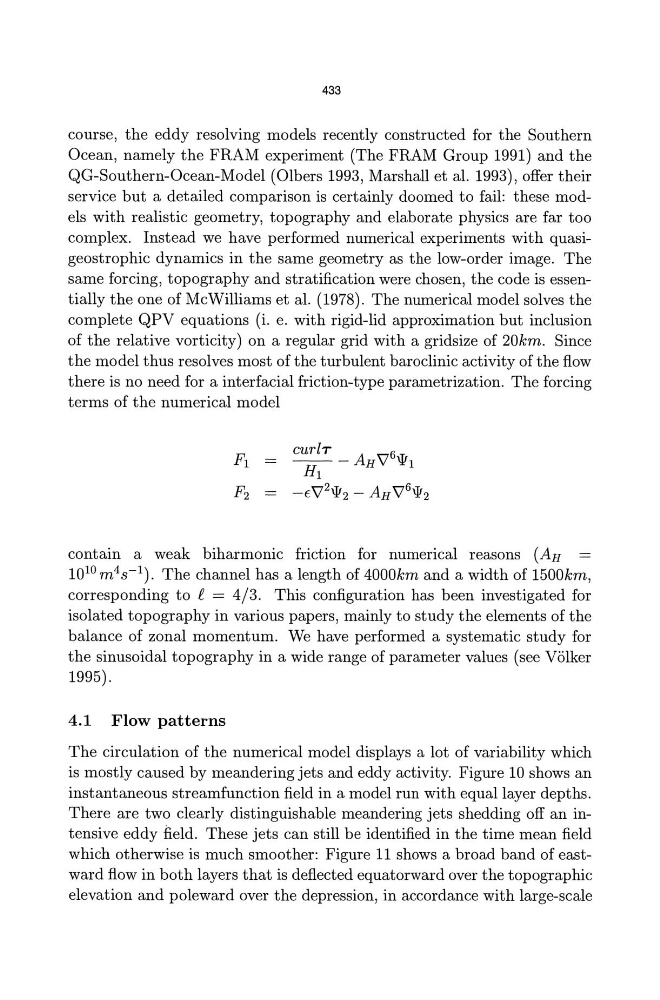
terms of the numerical model
contain a weak biharmonic friction for numerical reasons (AH
lO lD m 4 s- 1 ). The channel has a length of 4000km and a width of 1500km,
corresponding to £ = 4/3. This configuration has been investigated for
isolated topography in various papers, mainly to study the elements of the
balance of zonal momentum. We have performed a systematic study for
the sinusoidal topography in a wide range of parameter values (see Volker
1995).
4.1 Flow patterns
The circulation of the numerical model displays a lot of variability which
is mostly caused by meandering jets and eddy activity. Figure 10 shows an
instantaneous streamfunction field in a model run with equal layer depths.
There are two clearly distinguishable meandering jets shedding off an intensive eddy field. These jets can still be identified in the time mean field
which otherwise is much smoother: Figure 11 shows a broad band of eastward flow in both layers that is deflected equatorward over the topographic
elevation and poleward over the depression, in accordance with large-scale
course, the eddy resolving models recently constructed for the Southern
Ocean, namely the FRAM experiment (The FRAM Group 1991) and the
QG-Southern-Ocean-Model (Olbers 1993, Marshall et al. 1993), offer their
service but a detailed comparison is certainly doomed to fail: these models with realistic geometry, topography and elaborate physics are far too
complex. Instead we have performed numerical experiments with quasigeostrophic dynamics in the same geometry as the low-order image. The
same forcing, topography and stratification were chosen, the code is essentially the one of McWilliams et al. (1978). The numerical model solves the
complete QPV equations (i. e. with rigid-lid approximation but inclusion
of the relative vorticity) on a regular grid with a gridsize of 20km. Since
the model thus resolves most of the turbulent baroclinic activity of the flow
there is no need for a interfacial friction-type parametrization. The forcing
terms of the numerical model
contain a weak biharmonic friction for numerical reasons (AH
lO lD m 4 s- 1 ). The channel has a length of 4000km and a width of 1500km,
corresponding to £ = 4/3. This configuration has been investigated for
isolated topography in various papers, mainly to study the elements of the
balance of zonal momentum. We have performed a systematic study for
the sinusoidal topography in a wide range of parameter values (see Volker
1995).
4.1 Flow patterns
The circulation of the numerical model displays a lot of variability which
is mostly caused by meandering jets and eddy activity. Figure 10 shows an
instantaneous streamfunction field in a model run with equal layer depths.
There are two clearly distinguishable meandering jets shedding off an intensive eddy field. These jets can still be identified in the time mean field
which otherwise is much smoother: Figure 11 shows a broad band of eastward flow in both layers that is deflected equatorward over the topographic
elevation and poleward over the depression, in accordance with large-scale