366
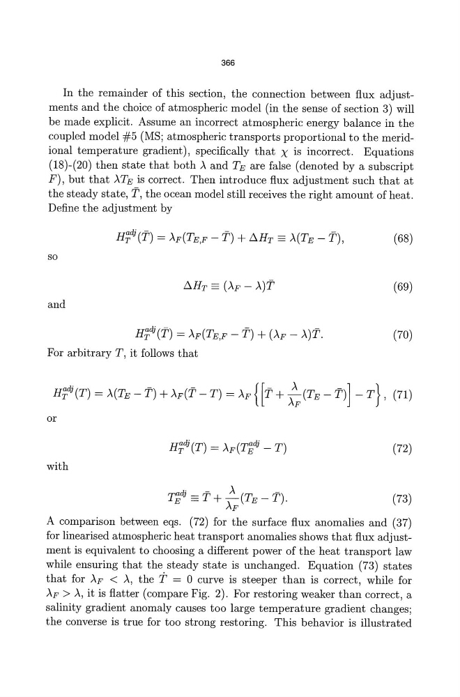
In the remainder of this section, the connection between flux adjustments and the choice of atmospheric model (in the sense of section 3) will
be made explicit. Assume an incorrect atmospheric energy balance in the
coupled model #5 (MS; atmospheric transports proportional to the meridional temperature gradient), specifically that X is incorrect. Equations
(18)-(20) then state that both A and TE are false (denoted by a subscript
F), but that ATE is correct. Then introduce flux adjustment such that at
the steady state, '1', the ocean model still receives the right amount of heat.
Define the adjustment by
d· -
-
-
H~1(T) = Ap(TE,P - T) + t::,.HT == A(TE - T),
(68)
so
(69)
and
d· -
-
-
H~1(T) = Ap(TE,p - T) + (Ap - A)T.
(70)
For arbitrary T, it follows that
H~dj (T) = A(TE - '1') + Ap('1' - T) = Ap {['1' + A~ (TE - '1')] - T}, (71)
or
(72)
with
(73)
A comparison between eqs. (72) for the surface flux anomalies and (37)
for linearised atmospheric heat transport anomalies shows that flux adjustment is equivalent to choosing a different power of the heat transport law
while ensuring that the steady state is unchanged. Equation (73) states
that for Ap < A, the T = 0 curve is steeper than is correct, while for
Ap > A, it is flatter (compare Fig. 2). For restoring weaker than correct, a
salinity gradient anomaly causes too large temperature gradient changes;
the converse is true for too strong restoring. This behavior is illustrated