360
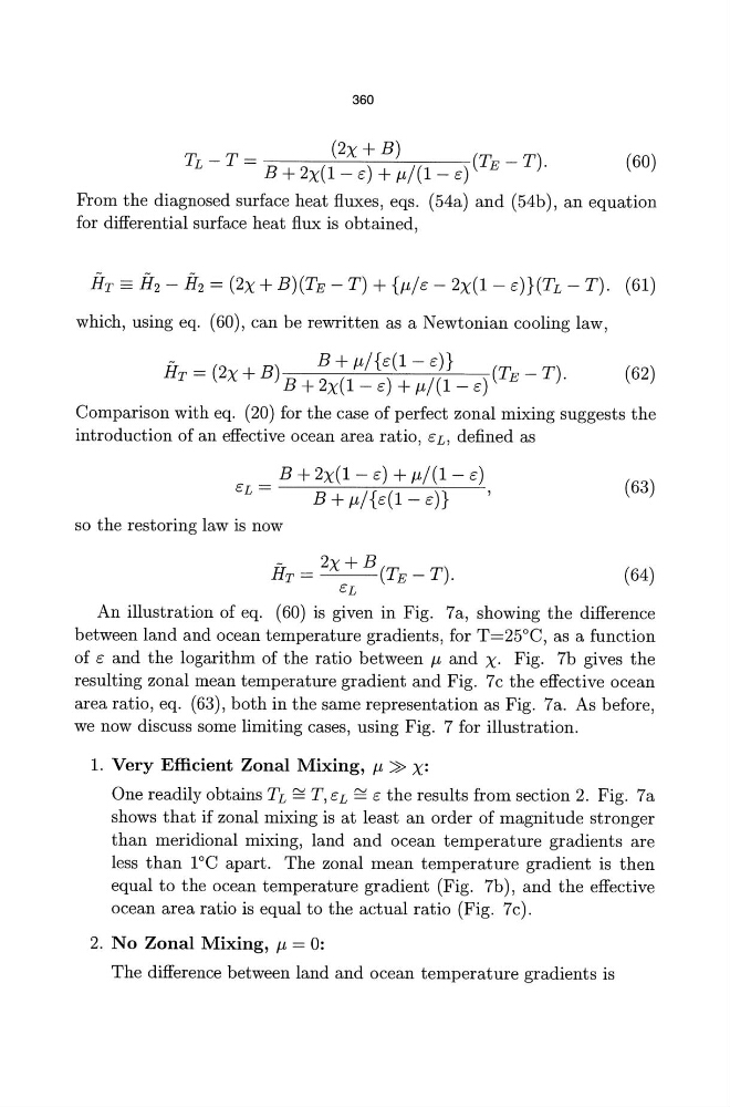
(60)
From the diagnosed surface heat fluxes, eqs. (54a) and (54b), an equation
for differential surface heat flux is obtained,
HT == H2 - H2 = (2X + B)(TE - T) + {/1,jE - 2X(1- E)}(TL - T). (61)
which, using eq. (60), can be rewritten as a Newtonian cooling law,
HT=(2X+B)
B+f-l/{E(l-E)}
(TE-T).
(62)
B + 2X(1 - E) + f-l/(1 - E)
Comparison with eq. (20) for the case of perfect zonal mixing suggests the
introduction of an effective ocean area ratio, EL, defined as
B + 2X(1 - E) + f-l/(1 - E)
EL -
-
B+f-l/{E(l-E)}
,
(63)
so the restoring law is now
(64)
An illustration of eq. (60) is given in Fig. 7a, showing the difference
between land and ocean temperature gradients, for T=25°C, as a function
of E and the logarithm of the ratio between f-l and X. Fig. 7b gives the
resulting zonal mean temperature gradient and Fig. 7c the effective ocean
area ratio, eq. (63), both in the same representation as Fig. 7a. As before,
we now discuss some limiting cases, using Fig. 7 for illustration.
1. Very Efficient Zonal Mixing, f-l» x:
One readily obtains TL ~ T, EL ~ E the results from section 2. Fig. 7a
shows that if zonal mixing is at least an order of magnitude stronger
than meridional mixing, land and ocean temperature gradients are
less than 1°C apart. The zonal mean temperature gradient is then
equal to the ocean temperature gradient (Fig. 7b), and the effective
ocean area ratio is equal to the actual ratio (Fig. 7c).
2. No Zonal Mixing, f-l = 0:
The difference between land and ocean temperature gradients is