

>
~
355
15.------r------~----~------~----_,
10 t:'"_ -:-_-' :::-_ -:-_-' ':-.:-_ -:-_-' =.:-:.0:-..... -.::." _. - . - ..
.......
.... ,
5
o
-5
\
\
\
\ ... - --10~----~----~----~------~----~
o
1000
2000
3000
4000
5000
Years
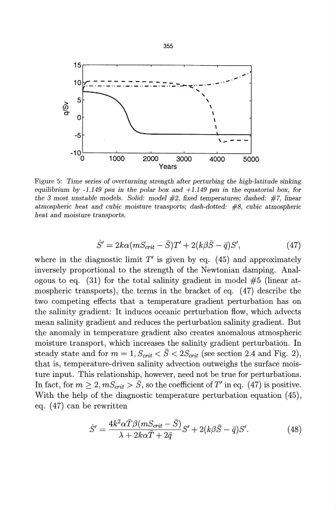
Figure 5: Time series of overturning strength after perturbing the high-latitude sinking
equilibrium by -1.149 psu in the polar box and +1.149 psu in the equatorial box, for
the 3 most unstable models. Solid: model #2, fixed temperatures; dashed: #7, linear
atmospheric heat and cubic moisture transports; dash-dotted: #8, cubic atmospheric
heat and moisture transports.
8' = 2ka(m8crit - S)T' + 2(k{3S - ij)8',
(47)
where in the diagnostic limit T' is given by eq. (45) and approximately
inversely proportional to the strength of the Newtonian damping. Analogous to eq. (31) for the total salinity gradient in model #5 (linear atmospheric transports), the terms in the bracket of eq. (47) describe the
two competing effects that a temperature gradient perturbation has on
the salinity gradient: It induces oceanic perturbation flow, which advects
mean salinity gradient and reduces the perturbation salinity gradient. But
the anomaly in temperature gradient also creates anomalous atmospheric
moisture transport, which increases the salinity gradient perturbation. In
steady state and for m = 1, 8 crit < S < 28crit (see section 2.4 and Fig. 2),
that is, temperature-driven salinity advection outweighs the surface moisture input. This relationship, however, need not be true for perturbations.
In fact, for m ~ 2, m8crit > S, so the coefficient ofT' in eq. (47) is positive.
With the help of the diagnostic temperature perturbation equation (45),
eq. (47) can be rewritten
8' = 4k
2
aT{3( m8 crit - S) 8' 2(k{3S - -)8'.
oX + 2kaT + 2ij
+
q
(48)
~
355
15.------r------~----~------~----_,
10 t:'"_ -:-_-' :::-_ -:-_-' ':-.:-_ -:-_-' =.:-:.0:-..... -.::." _. - . - ..
.......
.... ,
5
o
-5
\
\
\
\ ... - --10~----~----~----~------~----~
o
1000
2000
3000
4000
5000
Years
Figure 5: Time series of overturning strength after perturbing the high-latitude sinking
equilibrium by -1.149 psu in the polar box and +1.149 psu in the equatorial box, for
the 3 most unstable models. Solid: model #2, fixed temperatures; dashed: #7, linear
atmospheric heat and cubic moisture transports; dash-dotted: #8, cubic atmospheric
heat and moisture transports.
8' = 2ka(m8crit - S)T' + 2(k{3S - ij)8',
(47)
where in the diagnostic limit T' is given by eq. (45) and approximately
inversely proportional to the strength of the Newtonian damping. Analogous to eq. (31) for the total salinity gradient in model #5 (linear atmospheric transports), the terms in the bracket of eq. (47) describe the
two competing effects that a temperature gradient perturbation has on
the salinity gradient: It induces oceanic perturbation flow, which advects
mean salinity gradient and reduces the perturbation salinity gradient. But
the anomaly in temperature gradient also creates anomalous atmospheric
moisture transport, which increases the salinity gradient perturbation. In
steady state and for m = 1, 8 crit < S < 28crit (see section 2.4 and Fig. 2),
that is, temperature-driven salinity advection outweighs the surface moisture input. This relationship, however, need not be true for perturbations.
In fact, for m ~ 2, m8crit > S, so the coefficient ofT' in eq. (47) is positive.
With the help of the diagnostic temperature perturbation equation (45),
eq. (47) can be rewritten
8' = 4k
2
aT{3( m8 crit - S) 8' 2(k{3S - -)8'.
oX + 2kaT + 2ij
+
q
(48)