

353
Model #
Definition
t::..Sc
t::..Sc
Case 1: Case 2:
1
Fixed surface flux
00
00
3
Xo, 'Yo, radiative restoring
2.4
1.9
4
Xl, 'Yo, diffusive + fixed E-P
1.8
1.4
5
X1,'Y1, MS
1.6
1.2
6
X3, ' Y1
1.4
1.0
8
X3, 'Y3, ~ NSM
1.150
0.73
7
Xl, ' Y3
1.149
0.68
2
Fixed temperatures
1.13
0.77
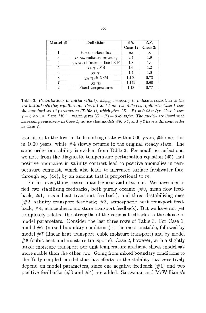
Table 3: Perturbations in initial salinity, t::..Scrit, necessary to induce a transition to the
low-latitude sinking equilibrium. Cases 1 and 2 are two different equilibria; Case 1 uses
the standard set of parameters (Table 1), which gives (E - P) = 0.42 m/yr. Case 2 uses
'Y = 3.2 X 10- 10 ms- 1 K- 1 , which gives (E - P) = 0.49 m/yr. The models are listed with
increasing sensitivity in Case 1; notice that models #8, #7, and #2 have a different order
in Case 2.
transition to the low-latitude sinking state within 500 years, #5 does this
in 1000 years, while #4 slowly returns to the original steady state. The
same order in stability is evident from Table 3. For small perturbations,
we note from the diagnostic temperature perturbation equation (45) that
positive anomalies in salinity contrast lead to positive anomalies in temperature contrast, which also leads to increased surface freshwater flux,
through eq. (44), by an amount that is proportional to m.
So far, everything seems unambiguous and clear-cut. We have identified two stabilising feedbacks, both purely oceanic (#0, mean flow feedback; #1, ocean heat transport feedback), and three destabilising ones
(#2, salinity transport feedback; #3, atmospheric heat transport feedback; #4, atmospheric moisture transport feedback). But we have not yet
completely related the strengths of the various feedbacks to the choice of
model parameters. Consider the last three rows of Table 3. For Case 1,
model #2 (mixed boundary conditions) is the most unstable, followed by
model #7 (linear heat transport, cubic moisture transport) and by model
#8 (cubic heat and moisture transports). Case 2, however, with a slightly
larger moisture transport per unit temperature gradient, shows model #2
more stable than the other two. Going from mixed boundary conditions to
the 'fully coupled' model thus has effects on the stability that sensitively
depend on model parameters, since one negative feedback (#1) and two
positive feedbacks (#3 and #4) are added. Saravanan and McWilliams's
Model #
Definition
t::..Sc
t::..Sc
Case 1: Case 2:
1
Fixed surface flux
00
00
3
Xo, 'Yo, radiative restoring
2.4
1.9
4
Xl, 'Yo, diffusive + fixed E-P
1.8
1.4
5
X1,'Y1, MS
1.6
1.2
6
X3, ' Y1
1.4
1.0
8
X3, 'Y3, ~ NSM
1.150
0.73
7
Xl, ' Y3
1.149
0.68
2
Fixed temperatures
1.13
0.77
Table 3: Perturbations in initial salinity, t::..Scrit, necessary to induce a transition to the
low-latitude sinking equilibrium. Cases 1 and 2 are two different equilibria; Case 1 uses
the standard set of parameters (Table 1), which gives (E - P) = 0.42 m/yr. Case 2 uses
'Y = 3.2 X 10- 10 ms- 1 K- 1 , which gives (E - P) = 0.49 m/yr. The models are listed with
increasing sensitivity in Case 1; notice that models #8, #7, and #2 have a different order
in Case 2.
transition to the low-latitude sinking state within 500 years, #5 does this
in 1000 years, while #4 slowly returns to the original steady state. The
same order in stability is evident from Table 3. For small perturbations,
we note from the diagnostic temperature perturbation equation (45) that
positive anomalies in salinity contrast lead to positive anomalies in temperature contrast, which also leads to increased surface freshwater flux,
through eq. (44), by an amount that is proportional to m.
So far, everything seems unambiguous and clear-cut. We have identified two stabilising feedbacks, both purely oceanic (#0, mean flow feedback; #1, ocean heat transport feedback), and three destabilising ones
(#2, salinity transport feedback; #3, atmospheric heat transport feedback; #4, atmospheric moisture transport feedback). But we have not yet
completely related the strengths of the various feedbacks to the choice of
model parameters. Consider the last three rows of Table 3. For Case 1,
model #2 (mixed boundary conditions) is the most unstable, followed by
model #7 (linear heat transport, cubic moisture transport) and by model
#8 (cubic heat and moisture transports). Case 2, however, with a slightly
larger moisture transport per unit temperature gradient, shows model #2
more stable than the other two. Going from mixed boundary conditions to
the 'fully coupled' model thus has effects on the stability that sensitively
depend on model parameters, since one negative feedback (#1) and two
positive feedbacks (#3 and #4) are added. Saravanan and McWilliams's