312
Coupling strategy (ECHAM4/ OPYC3)
- Ocean model_~---- Coupled mOICle. l-----If":"'±<~',l:(')1.~~. ~~~
spinup: 1000 years'
spinup: 100 years
~=e _(t/'t )2 ('t=5 years)
t=O
Fluxes of heat and freshwater
F=F A
F=FO
n
n = k f (FO-FA ) dn
o
time ___
t=100 years
AGCM
OGCM (incl. relax. towards SST OBS )
O = estimated from history of n
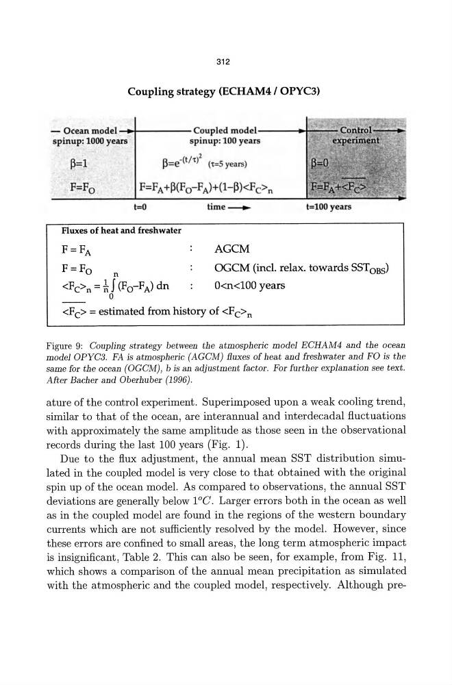
Figure 9: Coupling strategy between the atmospheric model ECHAM4 and the ocean
modelOPYC3, FA is atmospheric (AGCM) fluxes of heat and freshwater and FO is the
same for the ocean (OGCM) , b is an adjustment factor. For further explanation see text,
After Bacher and Oberhuber (1996) .
ature of the control experiment, Superimposed upon a weak cooling trend,
similar to that of the ocean, are interannual and interdecadal fluctuations
with approximately the same amplitude as those seen in the observational
records during the last 100 years (Fig. 1),
Due to the flux adjustment, the annual mean SST distribution simulated in the coupled model is very close to that obtained with the original
spin up of the ocean model. As compared to observations, the annual SST
deviations are generally below FG, Larger errors both in the ocean as well
as in the coupled model are found in the regions of the western boundary
currents which are not sufficiently resolved by the modeL However, since
these errors are confined to small areas, the long term atmospheric impact
is insignificant, Table 2. This can also be seen, for example, from Fig. 11 ,
which shows a comparison of the annual mean precipitation as simulated
with the atmospheric and the coupled model, respectively. Although pre-